1、2-17 实现多分类逻辑回归

代码

# 2-17 实现多分类逻辑回归
import pandas as pd
import numpy as np
import matplotlib.pyplot as plt

# 参数设置
iterations = 5400  # 迭代次数
learning_rate = 0.1  # 学习率
m_train = 200  # 训练样本数量


# 整数索引值转one-hot向量
def index2onehot(index, classes):
    onehot = np.zeros((classes, index.size))
    onehot[index.astype(int), np.arange(index.size)] = 1
    return onehot


# 读入轮椅数据
df = pd.read_csv('wheelchair_dataset.csv')
data = np.array(df)
m_all = np.shape(data)[0]  # 样本数量
d = np.shape(data)[1] - 1  # 输入特征维数
classes = np.amax(data[:, d])
m_test = m_all - m_train  # 测试样本的数量
# 构造随机种子为指定值的随机数生成器，并对数据集中样本随机排序
rng = np.random.default_rng(1)
rng.shuffle(data)
# 特征缩放（标准化）
data = data.astype(float)
mean = np.mean(data[0:m_train, 0:d], axis=0)
std = np.std(data[0:m_train, 0:d], axis=0, ddof=1)
data[:, 0:d] = (data[:, 0:d] - mean) / std
# 划分数据集
X_train = data[0:m_train, 0:d].T
Y_train = data[0:m_train, d].reshape((1, -1))
Y_train_onehot = index2onehot(Y_train.astype(int)-1, classes)  # 将类别标注值转为one-hot向量
X_test = data[m_train:, 0:d].T
Y_test = data[m_train, d].reshape((1, -1))
# 初始化
W = np.zeros((d, classes))
b = np.zeros((classes, 1))
v = np.ones((1, m_train))  # 1向量
U = np.ones((classes, classes))  # 1矩阵
costs_saved = []
# 迭代循环
for i in range(iterations):
    # 预测
    z = np.dot(W.T, X_train) + np.dot(b, v)
    exp_Z = np.exp(z)
    Y_hat = exp_Z / (np.dot(U, exp_Z))
    # 误差
    E = Y_hat - Y_train_onehot
    # 更新权重与偏差
    W = W - learning_rate * np.dot(X_train, E.T) / m_train  # 更新权重
    b = b - learning_rate * np.dot(E, v.T) / m_train  # 更新偏差
    # 保存代价函数的值
    costs = -np.trace(np.dot(Y_train_onehot.T, np.log(Y_hat))) / m_train
    costs_saved.append(costs.item(0))
#  打印最新权重与偏差
print('Weights=\n', np.array2string(W, precision=3))
print('Bias=', np.array2string(np.squeeze(b, axis=1), precision=3))
# 画代价函数值
plt.plot(range(1, np.size(costs_saved) + 1), costs_saved, 'r-o', linewidth=2, markersize=5)
plt.ylabel('costs')
plt.xlabel('iterations')
plt.title('learning rate=' + str(learning_rate))
plt.show()
# 训练数据集上的预测
z = np.dot(W.T, X_train) + b  # 广播操作
Y_train_hat = np.argmax(z, axis=0) + 1
# 测试数据集上的预测
z_test = np.dot(W.T, X_test) + b  # 广播操作
Y_test_hat = np.argmax(z_test, axis=0) + 1
# 分类错误数量
print('Trainset prediction errors=', np.sum(Y_train != Y_train_hat))
print('Testset prediction errors=', np.sum(Y_test != Y_test_hat))

结果图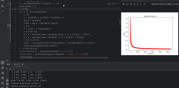

2、2-18实现二分类神经网络

代码

# 2-18 实现二分类神经网络
import pandas
import numpy as np
import matplotlib.pyplot as plt

# 参数设置
iterations = 1000  # 迭代次数
learning_rate = 0.1  # 学习率
m_train = 250  # 训练样本的数量
n = 2  # 隐含层节点的数量
# 读入酒驾检测数据集
df = pandas.read_csv('alcohol_dataset.csv')
data = np.array(df)
m_all = np.shape(data)[0]
d = np.shape(data)[1] - 1
m_test = m_all - m_train
# 构造随机种子为指定值的随机数生成器，并对数据集中的样本随机排序
rng = np.random.default_rng(1)
rng.shuffle(data)
# 标准化输入特征
mean = np.mean(data[0:m_train, 0:d], axis=0)
std = np.std(data[0:m_train, 0:d], axis=0, ddof=1)
data[:, 0:d] = (data[:, 0:d] - mean) / std
# 划分数据集
X_train = data[0:m_train, 0:d].T
X_test = data[m_train:, 0:d].T
y_train = data[0:m_train, d].reshape((1, -1))
y_test = data[m_train:, d].reshape((1, -1))
# 初始化
W_1 = rng.random((d, n))  # W[1]
b_1 = rng.random((n, 1))  # b[1]
w_2 = rng.random((n, 1))  # w[2]
b_2 = rng.random()  # b[2]
v = np.ones((1, m_train)).reshape((1, -1))  # v
costs_saved = []
for i in range(iterations):
    # 正向传播
    Z_1 = np.dot(W_1.T, X_train) + np.dot(b_1, v)
    A_1 = Z_1 * (Z_1 > 0)
    z_2 = np.dot(w_2.T, A_1) + b_2 * v
    y_hat = 1. / (1. + np.exp(-z_2))
    # 反向传播
    e = y_hat - y_train
    db_2 = np.dot(v, e.T) / m_train
    dw_2 = np.dot(A_1, e.T) / m_train
    db_1 = np.dot(w_2 * (Z_1 > 0), e.T) / m_train
    dW_1_dot = np.dot(w_2, e) * (Z_1 > 0)
    dW_1 = np.dot(X_train, dW_1_dot.T) / m_train
    # 更新权重与偏差参数
    b_1 = b_1 - learning_rate * db_1
    W_1 = W_1 - learning_rate * dW_1
    b_2 = b_2 - learning_rate * db_2
    w_2 = w_2 - learning_rate * dw_2
    # 保存代价函数的值
    costs = - (np.dot(np.log(y_hat), y_train.T) + np.dot(np.log(1 - y_hat), (1 - y_train).T)) / m_train
    costs_saved.append(costs.item(0))
# 打印最新权重与偏差
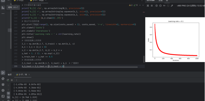
print('W_[1] =\n', np.array2string(W_1, precision=3))
print('b_[1] =', np.array2string(np.squeeze(b_1, axis=1), precision=3))
print('w_[2] =', np.array2string(np.squeeze(w_2, axis=1), precision=3))
print(f'b_[2] = {b_2.item(0):.3f}')
# 画出代价函数的值
plt.plot(range(1, np.size(costs_saved) + 1), costs_saved, 'r-o', linewidth=2, markersize=5)
plt.ylabel('Costs')
plt.xlabel('Iterations')
plt.title('Learning rate = ' + str(learning_rate))
plt.show()
# 训练数据集上的预测
Z_1 = np.dot(W_1.T, X_train) + np.dot(b_1, v)
A_1 = Z_1 * (Z_1 > 0)
z_2 = np.dot(w_2.T, A_1) + b_2 * v
y_hat = 1. / (1. + np.exp(-z_2))
y_train_hat = y_hat >= 0.5
# 测试数据集上的预测
Z_1_test = np.dot(W_1.T, X_test) + b_1  # 广播操作
A_1_test = Z_1_test * (Z_1_test > 0)
z_2_test = np.dot(w_2.T, A_1_test) + b_2  # 广播操作
y_hat_test = 1. / (1. + np.exp(-z_2_test))
y_test_hat = y_hat_test >= 0.5
# 打印预测错误数量
print('Trainset prediction errors =', np.sum(y_train != y_train_hat))
print('Testset prediction errors =', np.sum(y_test != y_test_hat))

结果图