@浙大疏锦行
早停策略和模型权重的保存
作业:对信贷数据集训练后保存权重,加载权重后继续训练50轮,并采取早停策略
import torch
import torch.nn as nn
import pandas as pd
import matplotlib.pyplot as plt
import torch.optim as optim
from sklearn.model_selection import train_test_split
from sklearn.preprocessing import MinMaxScaler
import time
import warnings
from tqdm import tqdm
warnings.filterwarnings("ignore")

# 设置GPU设备
device = torch.device("cuda:0" if torch.cuda.is_available() else "cpu")
print(f"使用设备: {device}")

# 设置中文字体
plt.rcParams['font.sans-serif'] = ['SimHei']
plt.rcParams['axes.unicode_minus'] = False

# 数据预处理部分(保持不变)
data = pd.read_csv('data.csv')

# 处理分类特征
discrete_features = data.select_dtypes(include=['object']).columns.tolist()

home_ownership_mapping = {
    'Own Home': 1,
    'Rent': 2,
    'Have Mortgage': 3,
    'Home Mortgage': 4
}
data['Home Ownership'] = data['Home Ownership'].map(home_ownership_mapping)

years_in_job_mapping = {
    '< 1 year': 1,
    '1 year': 2,
    '2 years': 3,
    '3 years': 4,
    '4 years': 5,
    '5 years': 6,
    '6 years': 7,
    '7 years': 8,
    '8 years': 9,
    '9 years': 10,
    '10+ years': 11
}
data['Years in current job'] = data['Years in current job'].map(years_in_job_mapping)

data = pd.get_dummies(data, columns=['Purpose'])
data2 = pd.read_csv("data.csv")
list_final = []
for i in data.columns:
    if i not in data2.columns:
        list_final.append(i)
for i in list_final:
    data[i] = data[i].astype(int)

term_mapping = {
    'Short Term': 0,
    'Long Term': 1
}
data['Term'] = data['Term'].map(term_mapping)
data.rename(columns={'Term': 'Long Term'}, inplace=True)

continuous_features = data.select_dtypes(include=['int64', 'float64']).columns.tolist()

# 缺失值处理
for feature in continuous_features:
    mode_value = data[feature].mode()[0]
    data[feature].fillna(mode_value, inplace=True)

# 数据集划分
X = data.drop(['Credit Default'], axis=1)
y = data['Credit Default']
X_train, X_test, y_train, y_test = train_test_split(X, y, test_size=0.2, random_state=42)

# 归一化数据
scaler = MinMaxScaler()
X_train = scaler.fit_transform(X_train)
X_test = scaler.transform(X_test)

# 转换为PyTorch张量
X_train = torch.FloatTensor(X_train).to(device)
y_train = torch.LongTensor(y_train.values).to(device)
X_test = torch.FloatTensor(X_test).to(device)
y_test = torch.LongTensor(y_test.values).to(device)

# 定义模型
class MLP(nn.Module):
    def __init__(self):
        super(MLP, self).__init__()
        self.fc1 = nn.Linear(31, 10)
        self.relu = nn.ReLU()
        self.fc2 = nn.Linear(10, 3)

    def forward(self, x):
        out = self.fc1(x)
        out = self.relu(out)
        out = self.fc2(out)
        return out

# 保存训练状态的函数
def save_checkpoint(model, optimizer, epoch, train_losses, test_losses, epochs, best_test_loss, best_epoch, counter, path):
    checkpoint = {
        'model_state_dict': model.state_dict(),
        'optimizer_state_dict': optimizer.state_dict(),
        'epoch': epoch,
        'train_losses': train_losses,
        'test_losses': test_losses,
        'epochs': epochs,
        'best_test_loss': best_test_loss,
        'best_epoch': best_epoch,
        'counter': counter
    }
    torch.save(checkpoint, path)

# 加载训练状态的函数
def load_checkpoint(model, optimizer, path):
    checkpoint = torch.load(path)
    model.load_state_dict(checkpoint['model_state_dict'])
    optimizer.load_state_dict(checkpoint['optimizer_state_dict'])
    epoch = checkpoint['epoch']
    train_losses = checkpoint['train_losses']
    test_losses = checkpoint['test_losses']
    epochs = checkpoint['epochs']
    best_test_loss = checkpoint['best_test_loss']
    best_epoch = checkpoint['best_epoch']
    counter = checkpoint['counter']
    return model, optimizer, epoch, train_losses, test_losses, epochs, best_test_loss, best_epoch, counter

# 主训练逻辑
def train_model(model, optimizer, criterion, X_train, y_train, X_test, y_test,
                start_epoch=0, num_epochs=20000, patience=50, checkpoint_path=None,
                continue_training=False):

    # 初始化训练历史
    if continue_training:
        model, optimizer, start_epoch, train_losses, test_losses, epochs, best_test_loss, best_epoch, counter = load_checkpoint(
            model, optimizer, checkpoint_path)
        print(f"从第 {start_epoch+1} 轮开始继续训练")
    else:
        train_losses = []
        test_losses = []
        epochs = []
        best_test_loss = float('inf')
        best_epoch = 0
        counter = 0
        print("开始全新训练")

    # 早停参数
    early_stopped = False

    start_time = time.time()

    # 创建tqdm进度条
    with tqdm(total=num_epochs, initial=start_epoch, desc="训练进度", unit="epoch") as pbar:
        for epoch in range(start_epoch, num_epochs):
            # 前向传播
            outputs = model(X_train)
            train_loss = criterion(outputs, y_train)

            # 反向传播和优化
            optimizer.zero_grad()
            train_loss.backward()
            optimizer.step()

            # 记录损失值
            if (epoch + 1) % 200 == 0:
                # 计算测试集损失
                model.eval()
                with torch.no_grad():
                    test_outputs = model(X_test)
                    test_loss = criterion(test_outputs, y_test)
                model.train()

                train_losses.append(train_loss.item())
                test_losses.append(test_loss.item())
                epochs.append(epoch + 1)

                # 更新进度条
                pbar.set_postfix({'Train Loss': f'{train_loss.item():.4f}', 'Test Loss': f'{test_loss.item():.4f}'})

                # 早停逻辑
                if test_loss.item() < best_test_loss:
                    best_test_loss = test_loss.item()
                    best_epoch = epoch + 1
                    counter = 0
                    # 保存最佳模型
                    torch.save(model.state_dict(), 'best_model.pth')
                    print(f"在第 {epoch+1} 轮保存了最佳模型,测试损失: {best_test_loss:.4f}")
                else:
                    counter += 1
                    if counter >= patience:
                        print(f"早停触发!在第{epoch+1}轮,测试集损失已有{patience}轮未改善。")
                        print(f"最佳测试集损失出现在第{best_epoch}轮,损失值为{best_test_loss:.4f}")
                        early_stopped = True
                        break

                # 保存检查点
                save_checkpoint(model, optimizer, epoch+1, train_losses, test_losses, epochs,
                                best_test_loss, best_epoch, counter, 'checkpoint.pth')

            # 每1000个epoch更新一次进度条
            if (epoch + 1) % 1000 == 0:
                pbar.update(1000)

        # 确保进度条达到100%
        if pbar.n < num_epochs:
            pbar.update(num_epochs - pbar.n)

    time_all = time.time() - start_time
    print(f'Training time: {time_all:.2f} seconds')

    return model, train_losses, test_losses, epochs, best_test_loss, best_epoch, early_stopped

# 主程序
if __name__ == "__main__":
    # 实例化模型
    model = MLP().to(device)

    # 定义损失函数和优化器
    criterion = nn.CrossEntropyLoss()
    optimizer = optim.SGD(model.parameters(), lr=0.01)

    # 第一阶段训练
    print("===== 第一阶段训练 =====")
    model, train_losses1, test_losses1, epochs1, best_test_loss1, best_epoch1, early_stopped1 = train_model(
        model, optimizer, criterion, X_train, y_train, X_test, y_test,
        num_epochs=20000, patience=50, checkpoint_path='checkpoint.pth', continue_training=False)

    # 加载最佳模型进行评估
    model.load_state_dict(torch.load('best_model.pth'))
    model.eval()
    with torch.no_grad():
        outputs = model(X_test)
        _, predicted = torch.max(outputs, 1)
        correct = (predicted == y_test).sum().item()
        accuracy = correct / y_test.size(0)
        print(f'第一阶段测试集准确率: {accuracy * 100:.2f}%')

    # 第二阶段训练:加载权重继续训练50轮,并采用早停策略
    print("\n===== 第二阶段训练:加载权重继续训练50轮 =====")
    # 重新实例化模型
    model_continued = MLP().to(device)
    # 加载最佳权重
    model_continued.load_state_dict(torch.load('best_model.pth'))
    # 重置优化器(可选)
    optimizer_continued = optim.SGD(model_continued.parameters(), lr=0.01)

    # 继续训练50轮
    model_continued, train_losses2, test_losses2, epochs2, best_test_loss2, best_epoch2, early_stopped2 = train_model(
        model_continued, optimizer_continued, criterion, X_train, y_train, X_test, y_test,
        start_epoch=0, num_epochs=50, patience=10, checkpoint_path='checkpoint_continued.pth', continue_training=False)

    # 最终评估
    model_continued.eval()
    with torch.no_grad():
        outputs = model_continued(X_test)
        _, predicted = torch.max(outputs, 1)
        correct = (predicted == y_test).sum().item()
        accuracy = correct / y_test.size(0)
        print(f'第二阶段测试集准确率: {accuracy * 100:.2f}%')

    # 合并损失曲线数据
    all_epochs = epochs1 + [e + epochs1[-1] if epochs1 else e for e in epochs2]
    all_train_losses = train_losses1 + train_losses2
    all_test_losses = test_losses1 + test_losses2

    # 可视化合并的损失曲线
    plt.figure(figsize=(12, 6))
    plt.plot(all_epochs, all_train_losses, label='Train Loss')
    plt.plot(all_epochs, all_test_losses, label='Test Loss')
    plt.axvline(x=epochs1[-1] if epochs1 else 0, color='r', linestyle='--', label='模型加载点')
    plt.xlabel('Epoch')
    plt.ylabel('Loss')
    plt.title('完整训练过程的损失曲线')
    plt.legend()
    plt.grid(True)
    plt.show()
使用设备: cuda:0
===== 第一阶段训练 =====
开始全新训练
训练进度: 0%| | 0/20000 [00:00<?, ?epoch/s, Train Loss=0.7827, Test Loss=0.7925]在第 200 轮保存了最佳模型,测试损失: 0.7925
训练进度: 0%| | 0/20000 [00:00<?, ?epoch/s, Train Loss=0.6341, Test Loss=0.6490]在第 400 轮保存了最佳模型,测试损失: 0.6936
在第 600 轮保存了最佳模型,测试损失: 0.6490
训练进度: 0%| | 0/20000 [00:01<?, ?epoch/s, Train Loss=0.6062, Test Loss=0.6204]在第 800 轮保存了最佳模型,测试损失: 0.6204
训练进度: 5%|▌ | 1000/20000 [00:01<00:24, 777.06epoch/s, Train Loss=0.5706, Test Loss=0.5834]在第 1000 轮保存了最佳模型,测试损失: 0.5993
训练进度: 5%|▌ | 1000/20000 [00:01<00:24, 777.06epoch/s, Train Loss=0.5579, Test Loss=0.5703]在第 1200 轮保存了最佳模型,测试损失: 0.5834
在第 1400 轮保存了最佳模型,测试损失: 0.5703
训练进度: 5%|▌ | 1000/20000 [00:02<00:24, 777.06epoch/s, Train Loss=0.5374, Test Loss=0.5488]在第 1600 轮保存了最佳模型,测试损失: 0.5589
在第 1800 轮保存了最佳模型,测试损失: 0.5488
训练进度: 10%|█ | 2000/20000 [00:02<00:20, 865.72epoch/s, Train Loss=0.5214, Test Loss=0.5318]在第 2000 轮保存了最佳模型,测试损失: 0.5398
训练进度: 10%|█ | 2000/20000 [00:02<00:20, 865.72epoch/s, Train Loss=0.5147, Test Loss=0.5248]在第 2200 轮保存了最佳模型,测试损失: 0.5318
在第 2400 轮保存了最佳模型,测试损失: 0.5248
训练进度: 10%|█ | 2000/20000 [00:03<00:20, 865.72epoch/s, Train Loss=0.5039, Test Loss=0.5133]在第 2600 轮保存了最佳模型,测试损失: 0.5186
训练进度: 10%|█ | 2000/20000 [00:03<00:20, 865.72epoch/s, Train Loss=0.4996, Test Loss=0.5088]在第 2800 轮保存了最佳模型,测试损失: 0.5133
训练进度: 15%|█▌ | 3000/20000 [00:03<00:18, 941.13epoch/s, Train Loss=0.4959, Test Loss=0.5049]在第 3000 轮保存了最佳模型,测试损失: 0.5088
训练进度: 15%|█▌ | 3000/20000 [00:03<00:18, 941.13epoch/s, Train Loss=0.4927, Test Loss=0.5015]在第 3200 轮保存了最佳模型,测试损失: 0.5049
训练进度: 15%|█▌ | 3000/20000 [00:03<00:18, 941.13epoch/s, Train Loss=0.4900, Test Loss=0.4987]在第 3400 轮保存了最佳模型,测试损失: 0.5015
在第 3600 轮保存了最佳模型,测试损失: 0.4987
训练进度: 15%|█▌ | 3000/20000 [00:04<00:18, 941.13epoch/s, Train Loss=0.4856, Test Loss=0.4941]在第 3800 轮保存了最佳模型,测试损失: 0.4962
训练进度: 20%|██ | 4000/20000 [00:04<00:16, 974.43epoch/s, Train Loss=0.4839, Test Loss=0.4923]在第 4000 轮保存了最佳模型,测试损失: 0.4941
训练进度: 20%|██ | 4000/20000 [00:04<00:16, 974.43epoch/s, Train Loss=0.4824, Test Loss=0.4907]在第 4200 轮保存了最佳模型,测试损失: 0.4923
训练进度: 20%|██ | 4000/20000 [00:04<00:16, 974.43epoch/s, Train Loss=0.4810, Test Loss=0.4894]在第 4400 轮保存了最佳模型,测试损失: 0.4907
训练进度: 20%|██ | 4000/20000 [00:05<00:16, 974.43epoch/s, Train Loss=0.4799, Test Loss=0.4882]在第 4600 轮保存了最佳模型,测试损失: 0.4894
训练进度: 20%|██ | 4000/20000 [00:05<00:16, 974.43epoch/s, Train Loss=0.4788, Test Loss=0.4871]在第 4800 轮保存了最佳模型,测试损失: 0.4882
训练进度: 25%|██▌ | 5000/20000 [00:05<00:15, 999.44epoch/s, Train Loss=0.4788, Test Loss=0.4871]在第 5000 轮保存了最佳模型,测试损失: 0.4871
训练进度: 25%|██▌ | 5000/20000 [00:05<00:15, 999.44epoch/s, Train Loss=0.4771, Test Loss=0.4853]在第 5200 轮保存了最佳模型,测试损失: 0.4861
在第 5400 轮保存了最佳模型,测试损失: 0.4853
训练进度: 25%|██▌ | 5000/20000 [00:06<00:15, 999.44epoch/s, Train Loss=0.4757, Test Loss=0.4838]在第 5600 轮保存了最佳模型,测试损失: 0.4845
训练进度: 30%|███ | 6000/20000 [00:06<00:14, 994.42epoch/s, Train Loss=0.4751, Test Loss=0.4831]在第 5800 轮保存了最佳模型,测试损失: 0.4838
在第 6000 轮保存了最佳模型,测试损失: 0.4831
训练进度: 30%|███ | 6000/20000 [00:06<00:14, 994.42epoch/s, Train Loss=0.4740, Test Loss=0.4820]在第 6200 轮保存了最佳模型,测试损失: 0.4825
训练进度: 30%|███ | 6000/20000 [00:06<00:14, 994.42epoch/s, Train Loss=0.4735, Test Loss=0.4815]在第 6400 轮保存了最佳模型,测试损失: 0.4820
训练进度: 30%|███ | 6000/20000 [00:07<00:14, 994.42epoch/s, Train Loss=0.4730, Test Loss=0.4810]在第 6600 轮保存了最佳模型,测试损失: 0.4815
训练进度: 35%|███▌ | 7000/20000 [00:07<00:12, 1005.58epoch/s, Train Loss=0.4726, Test Loss=0.4806]在第 6800 轮保存了最佳模型,测试损失: 0.4810
在第 7000 轮保存了最佳模型,测试损失: 0.4806
训练进度: 35%|███▌ | 7000/20000 [00:07<00:12, 1005.58epoch/s, Train Loss=0.4719, Test Loss=0.4798]在第 7200 轮保存了最佳模型,测试损失: 0.4802
训练进度: 35%|███▌ | 7000/20000 [00:07<00:12, 1005.58epoch/s, Train Loss=0.4715, Test Loss=0.4794]在第 7400 轮保存了最佳模型,测试损失: 0.4798
训练进度: 35%|███▌ | 7000/20000 [00:07<00:12, 1005.58epoch/s, Train Loss=0.4712, Test Loss=0.4791]在第 7600 轮保存了最佳模型,测试损失: 0.4794
在第 7800 轮保存了最佳模型,测试损失: 0.4791
训练进度: 40%|████ | 8000/20000 [00:08<00:12, 926.74epoch/s, Train Loss=0.4706, Test Loss=0.4785] 在第 8000 轮保存了最佳模型,测试损失: 0.4788
训练进度: 40%|████ | 8000/20000 [00:08<00:12, 926.74epoch/s, Train Loss=0.4703, Test Loss=0.4782]在第 8200 轮保存了最佳模型,测试损失: 0.4785
训练进度: 40%|████ | 8000/20000 [00:09<00:12, 926.74epoch/s, Train Loss=0.4701, Test Loss=0.4779]在第 8400 轮保存了最佳模型,测试损失: 0.4782
在第 8600 轮保存了最佳模型,测试损失: 0.4779
训练进度: 40%|████ | 8000/20000 [00:09<00:12, 926.74epoch/s, Train Loss=0.4696, Test Loss=0.4774]在第 8800 轮保存了最佳模型,测试损失: 0.4777
训练进度: 45%|████▌ | 9000/20000 [00:09<00:11, 940.37epoch/s, Train Loss=0.4696, Test Loss=0.4774]在第 9000 轮保存了最佳模型,测试损失: 0.4774
训练进度: 45%|████▌ | 9000/20000 [00:09<00:11, 940.37epoch/s, Train Loss=0.4691, Test Loss=0.4770]在第 9200 轮保存了最佳模型,测试损失: 0.4772
训练进度: 45%|████▌ | 9000/20000 [00:10<00:11, 940.37epoch/s, Train Loss=0.4689, Test Loss=0.4768]在第 9400 轮保存了最佳模型,测试损失: 0.4770
在第 9600 轮保存了最佳模型,测试损失: 0.4768
训练进度: 45%|████▌ | 9000/20000 [00:10<00:11, 940.37epoch/s, Train Loss=0.4685, Test Loss=0.4764]在第 9800 轮保存了最佳模型,测试损失: 0.4765
训练进度: 50%|█████ | 10000/20000 [00:10<00:10, 959.34epoch/s, Train Loss=0.4684, Test Loss=0.4762]在第 10000 轮保存了最佳模型,测试损失: 0.4764
训练进度: 50%|█████ | 10000/20000 [00:10<00:10, 959.34epoch/s, Train Loss=0.4682, Test Loss=0.4760]在第 10200 轮保存了最佳模型,测试损失: 0.4762
训练进度: 50%|█████ | 10000/20000 [00:11<00:10, 959.34epoch/s, Train Loss=0.4680, Test Loss=0.4758]在第 10400 轮保存了最佳模型,测试损失: 0.4760
在第 10600 轮保存了最佳模型,测试损失: 0.4758
训练进度: 50%|█████ | 10000/20000 [00:11<00:10, 959.34epoch/s, Train Loss=0.4677, Test Loss=0.4755]在第 10800 轮保存了最佳模型,测试损失: 0.4757
训练进度: 55%|█████▌ | 11000/20000 [00:11<00:09, 972.87epoch/s, Train Loss=0.4675, Test Loss=0.4754]在第 11000 轮保存了最佳模型,测试损失: 0.4755
训练进度: 55%|█████▌ | 11000/20000 [00:11<00:09, 972.87epoch/s, Train Loss=0.4674, Test Loss=0.4752]在第 11200 轮保存了最佳模型,测试损失: 0.4754
在第 11400 轮保存了最佳模型,测试损失: 0.4752
训练进度: 55%|█████▌ | 11000/20000 [00:12<00:09, 972.87epoch/s, Train Loss=0.4671, Test Loss=0.4749]在第 11600 轮保存了最佳模型,测试损失: 0.4751
训练进度: 55%|█████▌ | 11000/20000 [00:12<00:09, 972.87epoch/s, Train Loss=0.4669, Test Loss=0.4748]在第 11800 轮保存了最佳模型,测试损失: 0.4749
训练进度: 60%|██████ | 12000/20000 [00:12<00:08, 984.95epoch/s, Train Loss=0.4668, Test Loss=0.4747]在第 12000 轮保存了最佳模型,测试损失: 0.4748
在第 12200 轮保存了最佳模型,测试损失: 0.4747
训练进度: 60%|██████ | 12000/20000 [00:13<00:08, 984.95epoch/s, Train Loss=0.4666, Test Loss=0.4744]在第 12400 轮保存了最佳模型,测试损失: 0.4746
在第 12600 轮保存了最佳模型,测试损失: 0.4744
训练进度: 60%|██████ | 12000/20000 [00:13<00:08, 984.95epoch/s, Train Loss=0.4663, Test Loss=0.4742]在第 12800 轮保存了最佳模型,测试损失: 0.4743
训练进度: 65%|██████▌ | 13000/20000 [00:13<00:07, 988.03epoch/s, Train Loss=0.4662, Test Loss=0.4741]在第 13000 轮保存了最佳模型,测试损失: 0.4742
训练进度: 65%|██████▌ | 13000/20000 [00:13<00:07, 988.03epoch/s, Train Loss=0.4661, Test Loss=0.4740]在第 13200 轮保存了最佳模型,测试损失: 0.4741
训练进度: 65%|██████▌ | 13000/20000 [00:14<00:07, 988.03epoch/s, Train Loss=0.4660, Test Loss=0.4739]在第 13400 轮保存了最佳模型,测试损失: 0.4740
在第 13600 轮保存了最佳模型,测试损失: 0.4739
训练进度: 65%|██████▌ | 13000/20000 [00:14<00:07, 988.03epoch/s, Train Loss=0.4658, Test Loss=0.4737]在第 13800 轮保存了最佳模型,测试损失: 0.4738
训练进度: 70%|███████ | 14000/20000 [00:14<00:06, 996.60epoch/s, Train Loss=0.4658, Test Loss=0.4737]在第 14000 轮保存了最佳模型,测试损失: 0.4737
训练进度: 70%|███████ | 14000/20000 [00:14<00:06, 996.60epoch/s, Train Loss=0.4657, Test Loss=0.4736]在第 14200 轮保存了最佳模型,测试损失: 0.4736
训练进度: 70%|███████ | 14000/20000 [00:14<00:06, 996.60epoch/s, Train Loss=0.4656, Test Loss=0.4735]在第 14400 轮保存了最佳模型,测试损失: 0.4735
训练进度: 70%|███████ | 14000/20000 [00:15<00:06, 996.60epoch/s, Train Loss=0.4655, Test Loss=0.4735]在第 14600 轮保存了最佳模型,测试损失: 0.4735
训练进度: 70%|███████ | 14000/20000 [00:15<00:06, 996.60epoch/s, Train Loss=0.4654, Test Loss=0.4734]在第 14800 轮保存了最佳模型,测试损失: 0.4734
训练进度: 75%|███████▌ | 15000/20000 [00:15<00:05, 904.70epoch/s, Train Loss=0.4653, Test Loss=0.4733]在第 15000 轮保存了最佳模型,测试损失: 0.4733
训练进度: 75%|███████▌ | 15000/20000 [00:16<00:05, 904.70epoch/s, Train Loss=0.4652, Test Loss=0.4732]在第 15200 轮保存了最佳模型,测试损失: 0.4732
训练进度: 75%|███████▌ | 15000/20000 [00:16<00:05, 904.70epoch/s, Train Loss=0.4651, Test Loss=0.4731]在第 15400 轮保存了最佳模型,测试损失: 0.4731
训练进度: 75%|███████▌ | 15000/20000 [00:16<00:05, 904.70epoch/s, Train Loss=0.4650, Test Loss=0.4731]在第 15600 轮保存了最佳模型,测试损失: 0.4731
训练进度: 75%|███████▌ | 15000/20000 [00:16<00:05, 904.70epoch/s, Train Loss=0.4649, Test Loss=0.4730]在第 15800 轮保存了最佳模型,测试损失: 0.4730
训练进度: 80%|████████ | 16000/20000 [00:17<00:04, 858.96epoch/s, Train Loss=0.4648, Test Loss=0.4729]在第 16000 轮保存了最佳模型,测试损失: 0.4729
训练进度: 80%|████████ | 16000/20000 [00:17<00:04, 858.96epoch/s, Train Loss=0.4648, Test Loss=0.4729]在第 16200 轮保存了最佳模型,测试损失: 0.4729
训练进度: 80%|████████ | 16000/20000 [00:17<00:04, 858.96epoch/s, Train Loss=0.4647, Test Loss=0.4728]在第 16400 轮保存了最佳模型,测试损失: 0.4728
训练进度: 80%|████████ | 16000/20000 [00:17<00:04, 858.96epoch/s, Train Loss=0.4646, Test Loss=0.4727]在第 16600 轮保存了最佳模型,测试损失: 0.4727
训练进度: 80%|████████ | 16000/20000 [00:18<00:04, 858.96epoch/s, Train Loss=0.4645, Test Loss=0.4727]在第 16800 轮保存了最佳模型,测试损失: 0.4727
训练进度: 85%|████████▌ | 17000/20000 [00:18<00:03, 836.11epoch/s, Train Loss=0.4644, Test Loss=0.4726]在第 17000 轮保存了最佳模型,测试损失: 0.4726
训练进度: 85%|████████▌ | 17000/20000 [00:18<00:03, 836.11epoch/s, Train Loss=0.4644, Test Loss=0.4725]在第 17200 轮保存了最佳模型,测试损失: 0.4725
训练进度: 85%|████████▌ | 17000/20000 [00:18<00:03, 836.11epoch/s, Train Loss=0.4643, Test Loss=0.4725]在第 17400 轮保存了最佳模型,测试损失: 0.4725
训练进度: 85%|████████▌ | 17000/20000 [00:19<00:03, 836.11epoch/s, Train Loss=0.4642, Test Loss=0.4724]在第 17600 轮保存了最佳模型,测试损失: 0.4724
训练进度: 85%|████████▌ | 17000/20000 [00:19<00:03, 836.11epoch/s, Train Loss=0.4642, Test Loss=0.4724]在第 17800 轮保存了最佳模型,测试损失: 0.4724
训练进度: 90%|█████████ | 18000/20000 [00:19<00:02, 798.55epoch/s, Train Loss=0.4641, Test Loss=0.4723]在第 18000 轮保存了最佳模型,测试损失: 0.4723
训练进度: 90%|█████████ | 18000/20000 [00:20<00:02, 798.55epoch/s, Train Loss=0.4640, Test Loss=0.4723]在第 18200 轮保存了最佳模型,测试损失: 0.4723
训练进度: 90%|█████████ | 18000/20000 [00:20<00:02, 798.55epoch/s, Train Loss=0.4640, Test Loss=0.4722]在第 18400 轮保存了最佳模型,测试损失: 0.4722
训练进度: 90%|█████████ | 18000/20000 [00:20<00:02, 798.55epoch/s, Train Loss=0.4639, Test Loss=0.4722]在第 18600 轮保存了最佳模型,测试损失: 0.4722
训练进度: 90%|█████████ | 18000/20000 [00:20<00:02, 798.55epoch/s, Train Loss=0.4639, Test Loss=0.4721]在第 18800 轮保存了最佳模型,测试损失: 0.4721
训练进度: 95%|█████████▌| 19000/20000 [00:21<00:01, 777.80epoch/s, Train Loss=0.4638, Test Loss=0.4721]在第 19000 轮保存了最佳模型,测试损失: 0.4721
训练进度: 95%|█████████▌| 19000/20000 [00:21<00:01, 777.80epoch/s, Train Loss=0.4637, Test Loss=0.4720]在第 19200 轮保存了最佳模型,测试损失: 0.4720
训练进度: 95%|█████████▌| 19000/20000 [00:21<00:01, 777.80epoch/s, Train Loss=0.4637, Test Loss=0.4720]在第 19400 轮保存了最佳模型,测试损失: 0.4720
训练进度: 95%|█████████▌| 19000/20000 [00:21<00:01, 777.80epoch/s, Train Loss=0.4636, Test Loss=0.4720]在第 19600 轮保存了最佳模型,测试损失: 0.4720
训练进度: 95%|█████████▌| 19000/20000 [00:22<00:01, 777.80epoch/s, Train Loss=0.4636, Test Loss=0.4719]在第 19800 轮保存了最佳模型,测试损失: 0.4719
训练进度: 100%|██████████| 20000/20000 [00:22<00:00, 893.30epoch/s, Train Loss=0.4635, Test Loss=0.4719]
在第 20000 轮保存了最佳模型,测试损失: 0.4719
Training time: 22.39 seconds
第一阶段测试集准确率: 77.00%
===== 第二阶段训练:加载权重继续训练50轮 =====
开始全新训练
训练进度: 100%|██████████| 50/50 [00:00<00:00, 446.66epoch/s]
Training time: 0.11 seconds
第二阶段测试集准确率: 77.00%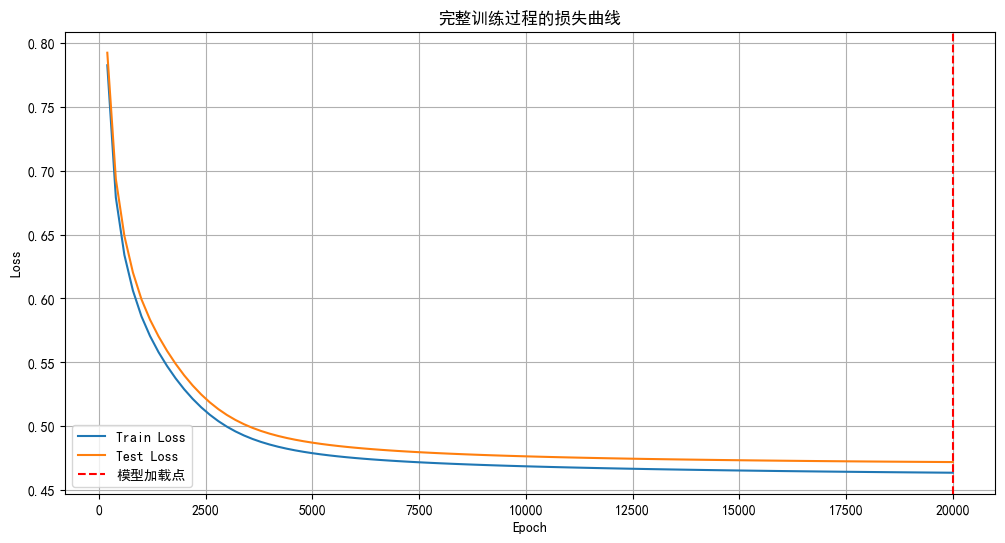


![[IMX] 08.RTC 时钟](https://i-blog.csdnimg.cn/direct/cf1619e0a2e64d79a8eb275406dc669e.png)