【NLP】使用 BERT 和 PyTorch Lightning 进行多标签文本分类

🔎大家好，我是Sonhhxg_柒，希望你看完之后，能对你有所帮助，不足请指正！共同学习交流🔎

📝个人主页－Sonhhxg_柒的博客_CSDN博客 📃

🎁欢迎各位→点赞👍 + 收藏⭐️ + 留言📝

📣系列专栏 - 机器学习【ML】自然语言处理【NLP】深度学习【DL】

🖍foreword

✔说明⇢本人讲解主要包括Python、机器学习（ML）、深度学习（DL）、自然语言处理（NLP）等内容。

如果你对这个系列感兴趣的话，可以关注订阅哟👋

文章目录

数据

预处理

Tokenization

数据集

模型

优化器调度器

评估

训练

预测

评估

概括

了解如何为多标签文本分类（标记）准备带有恶意评论的数据集。我们将使用 PyTorch Lightning 微调 BERT 并评估模型。

多标签文本分类（或标记文本）是您在执行 NLP 时会遇到的最常见任务之一。现代基于 Transformer 的模型（如 BERT）利用对大量文本数据的预训练，可以更快地进行微调，使用更少的资源并且在较小的（更）数据集上更准确。

在本教程中，您将学习如何：

将文本数据加载、平衡和拆分成集合
标记文本（使用 BERT 标记器）并创建 PyTorch 数据集
使用 PyTorch Lightning 微调 BERT 模型
了解热身步骤并使用学习率调度程序
在训练期间使用 ROC 下的面积和二元交叉熵来评估模型
如何使用微调的 BERT 模型进行预测
评估每个类的模型性能（可能的注释标记）

我们的模型对有害文本检测有用吗？

在浏览器中运行笔记本 (Google Colab)
阅读Getting Things Done with Pytorch一书

import pandas as pd
import numpy as np

from tqdm.auto import tqdm

import torch
import torch.nn as nn
from torch.utils.data import Dataset, DataLoader

from transformers import BertTokenizerFast as BertTokenizer, BertModel, AdamW, get_linear_schedule_with_warmup

import pytorch_lightning as pl
from pytorch_lightning.metrics.functional import accuracy, f1, auroc
from pytorch_lightning.callbacks import ModelCheckpoint, EarlyStopping
from pytorch_lightning.loggers import TensorBoardLogger

from sklearn.model_selection import train_test_split
from sklearn.metrics import classification_report, multilabel_confusion_matrix

import seaborn as sns
from pylab import rcParams
import matplotlib.pyplot as plt
from matplotlib import rc

%matplotlib inline
%config InlineBackend.figure_format='retina'

RANDOM_SEED = 42

sns.set(style='whitegrid', palette='muted', font_scale=1.2)
HAPPY_COLORS_PALETTE = ["#01BEFE", "#FFDD00", "#FF7D00", "#FF006D", "#ADFF02", "#8F00FF"]
sns.set_palette(sns.color_palette(HAPPY_COLORS_PALETTE))
rcParams['figure.figsize'] = 12, 8

pl.seed_everything(RANDOM_SEED)

数据

我们的数据集包含潜在的攻击性（有毒）评论，来自有毒评论分类挑战。让我们从下载数据开始（从 Google 云端硬盘）：

!gdown--ID1VQ-U7TtggShMeuRSA_hzC8qGDl2LRkr

让我们加载并查看数据：

df = pd.read_csv("toxic_comments.csv")
df.head()

	id	comment_text
0	0000997932d777bf	Explanation\nWhy the edits made under my usern...
1	000103f0d9cfb60f	D'aww! He matches this background colour I'm s...
2	000113f07ec002fd	Hey man, I'm really not trying to edit war. It...
3	0001b41b1c6bb37e	"\nMore\nI can't make any real suggestions on ...
4	0001d958c54c6e35	You, sir, are my hero. Any chance you remember...

我们有文字（评论）和六种不同的毒性标签。请注意，我们也有干净的内容。

让我们拆分数据：

train_df, val_df = train_test_split(df, test_size=0.05)
train_df.shape, val_df.shape

((151592, 8), (7979, 8))

预处理

让我们看看标签的分布：

LABEL_COLUMNS = df.columns.tolist()[2:]
df[LABEL_COLUMNS].sum().sort_values().plot(kind="barh");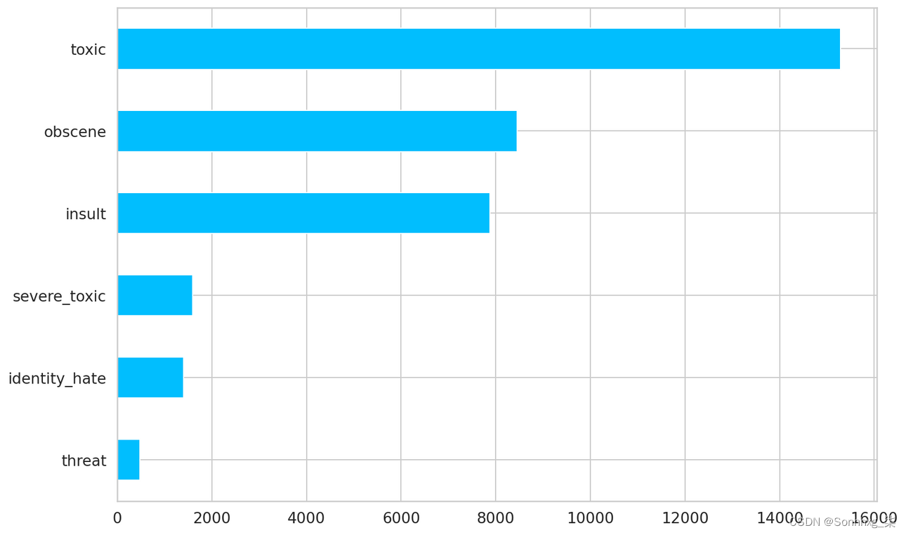

评论中的标签数量

我们有一个严重的失衡案例。但这还不是全部。有毒与干净的评论呢？

train_toxic = train_df[train_df[LABEL_COLUMNS].sum(axis=1) > 0]
train_clean = train_df[train_df[LABEL_COLUMNS].sum(axis=1) == 0]

pd.DataFrame(dict(
  toxic=[len(train_toxic)],
  clean=[len(train_clean)]
)).plot(kind='barh');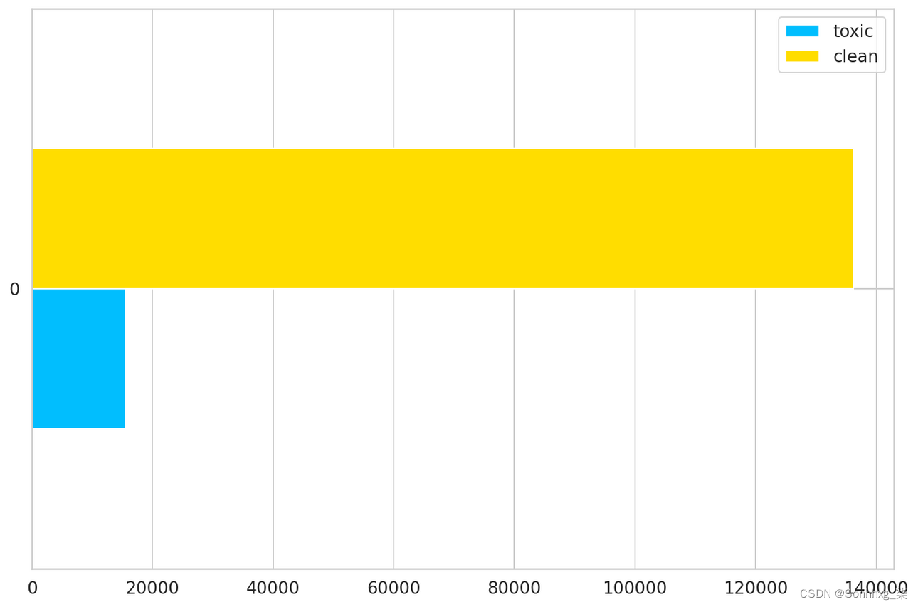

数据集中的干净评论与有毒评论计数

同样，我们对干净的评论存在严重的不平衡。为了解决这个问题，我们将从干净的评论中抽取 15,000 个示例并创建一个新的训练集：

train_df = pd.concat([
  train_toxic,
  train_clean.sample(15_000)
])

train_df.shape, val_df.shape

((30427, 8), (7979, 8))

Tokenization

我们需要将原始文本转换为标记列表。为此，我们将使用内置的 BertTokenizer：

BERT_MODEL_NAME = 'bert-base-cased'
tokenizer = BertTokenizer.from_pretrained(BERT_MODEL_NAME)

让我们在示例评论中尝试一下：

sample_row = df.iloc[16]
sample_comment = sample_row.comment_text
sample_labels = sample_row[LABEL_COLUMNS]

print(sample_comment)
print()
print(sample_labels.to_dict())

Bye!

Don't look, come or think of comming back! Tosser.

{'toxic': 1, 'severe_toxic': 0, 'obscene': 0, 'threat': 0, 'insult': 0, 'identity_hate': 0}

encoding = tokenizer.encode_plus(
  sample_comment,
  add_special_tokens=True,
  max_length=512,
  return_token_type_ids=False,
  padding="max_length",
  return_attention_mask=True,
  return_tensors='pt',
)

encoding.keys()

dict_keys(['input_ids', 'attention_mask'])

encoding["input_ids"].shape, encoding["attention_mask"].shape

(torch.Size([1, 512]), torch.Size([1, 512]))

编码的结果是一个带有标记 idinput_ids和注意力掩码的字典attention_mask（模型应该使用哪些标记 1 - 使用或 0 - 不使用）。

让我们看看它们的内容：

encoding["input_ids"].squeeze()[:20]

tensor([ 101, 17774, 106, 1790, 112, 189, 1440, 117, 1435, 1137,2 1341, 1104, 3254, 5031, 1171, 106, 1706, 14607, 119, 102])

encoding["attention_mask"].squeeze()[:20]

tensor([1, 1, 1, 1, 1, 1, 1, 1, 1, 1, 1, 1, 1, 1, 1, 1, 1, 1, 1, 1])

您还可以反转标记化并从标记 ID 中取回（有点）单词：

print(tokenizer.convert_ids_to_tokens(encoding["input_ids"].squeeze())[:20])

['[CLS]', 'Bye', '!', 'Don', "'", 't', 'look', ',', 'come', 'or', 'think', 'of', 'com', '##ming', 'back', '!', 'To', '##sser', '.', '[SEP]']

我们需要在编码时指定最大的标记数（512 是我们可以做的最大值）。让我们检查每个评论的标记数：

token_counts = []

for _, row in train_df.iterrows():
  token_count = len(tokenizer.encode(
    row["comment_text"],
    max_length=512,
    truncation=True
  ))
  token_counts.append(token_count)

sns.histplot(token_counts)
plt.xlim([0, 512]);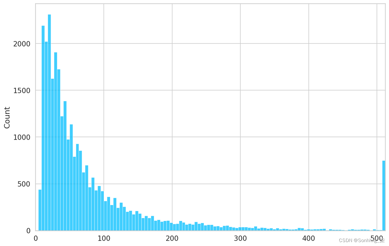

每条评论的标记数

大多数评论包含少于 300 个令牌或超过 512 个。因此，我们将坚持 512 个的限制。

MAX_TOKEN_COUNT = 512

数据集

我们将把标记化过程包装在 PyTorch 数据集中，同时将标签转换为张量：

class ToxicCommentsDataset(Dataset):

  def __init__(
    self,
    data: pd.DataFrame,
    tokenizer: BertTokenizer,
    max_token_len: int = 128
  ):
    self.tokenizer = tokenizer
    self.data = data
    self.max_token_len = max_token_len

  def __len__(self):
    return len(self.data)

  def __getitem__(self, index: int):
    data_row = self.data.iloc[index]

    comment_text = data_row.comment_text
    labels = data_row[LABEL_COLUMNS]

    encoding = self.tokenizer.encode_plus(
      comment_text,
      add_special_tokens=True,
      max_length=self.max_token_len,
      return_token_type_ids=False,
      padding="max_length",
      truncation=True,
      return_attention_mask=True,
      return_tensors='pt',
    )

    return dict(
      comment_text=comment_text,
      input_ids=encoding["input_ids"].flatten(),
      attention_mask=encoding["attention_mask"].flatten(),
      labels=torch.FloatTensor(labels)
    )

让我们看一下数据集中的示例项目：

train_dataset = ToxicCommentsDataset(
  train_df,
  tokenizer,
  max_token_len=MAX_TOKEN_COUNT
)

sample_item = train_dataset[0]
sample_item.keys()

dict_keys(['comment_text', 'input_ids', 'attention_mask', 'labels'])

sample_item["comment_text"]

'Hi, ya fucking idiot. ^_^'

sample_item["labels"]

tensor([1., 0., 1., 0., 1., 0.])

sample_item["input_ids"].shape

torch.Size([512])

让我们加载 BERT 模型并通过以下方式传递批处理数据样本：

bert_model = BertModel.from_pretrained(BERT_MODEL_NAME, return_dict=True)

sample_batch = next(iter(DataLoader(train_dataset, batch_size=8, num_workers=2)))
sample_batch["input_ids"].shape, sample_batch["attention_mask"].shape

(torch.Size([8, 512]), torch.Size([8, 512]))

output = bert_model(sample_batch["input_ids"], sample_batch["attention_mask"])

output.last_hidden_state.shape, output.pooler_output.shape

(torch.Size([8, 512, 768]), torch.Size([8, 768]))

维度来自768BERT hidden size：

bert_model.config.hidden_size

768

较大版本的 BERT 具有更多的注意力头和更大的隐藏尺寸。

我们会将自定义数据集包装到LightningDataModule中：

class ToxicCommentDataModule(pl.LightningDataModule):

  def __init__(self, train_df, test_df, tokenizer, batch_size=8, max_token_len=128):
    super().__init__()
    self.batch_size = batch_size
    self.train_df = train_df
    self.test_df = test_df
    self.tokenizer = tokenizer
    self.max_token_len = max_token_len

  def setup(self, stage=None):
    self.train_dataset = ToxicCommentsDataset(
      self.train_df,
      self.tokenizer,
      self.max_token_len
    )

    self.test_dataset = ToxicCommentsDataset(
      self.test_df,
      self.tokenizer,
      self.max_token_len
    )

  def train_dataloader(self):
    return DataLoader(
      self.train_dataset,
      batch_size=self.batch_size,
      shuffle=True,
      num_workers=2
    )

  def val_dataloader(self):
    return DataLoader(
      self.test_dataset,
      batch_size=self.batch_size,
      num_workers=2
    )

  def test_dataloader(self):
    return DataLoader(
      self.test_dataset,
      batch_size=self.batch_size,
      num_workers=2
    )

ToxicCommentDataModule封装所有数据加载逻辑并返回必要的数据加载器。让我们创建一个数据模块的实例：

N_EPOCHS = 10
BATCH_SIZE = 12

data_module = ToxicCommentDataModule(
  train_df,
  val_df,
  tokenizer,
  batch_size=BATCH_SIZE,
  max_token_len=MAX_TOKEN_COUNT
)

模型

我们的模型将使用预训练的BertModel和线性层将 BERT 表示转换为分类任务。我们会将所有内容打包到LightningModule中：

class ToxicCommentTagger(pl.LightningModule):

  def __init__(self, n_classes: int, n_training_steps=None, n_warmup_steps=None):
    super().__init__()
    self.bert = BertModel.from_pretrained(BERT_MODEL_NAME, return_dict=True)
    self.classifier = nn.Linear(self.bert.config.hidden_size, n_classes)
    self.n_training_steps = n_training_steps
    self.n_warmup_steps = n_warmup_steps
    self.criterion = nn.BCELoss()

  def forward(self, input_ids, attention_mask, labels=None):
    output = self.bert(input_ids, attention_mask=attention_mask)
    output = self.classifier(output.pooler_output)
    output = torch.sigmoid(output)
    loss = 0
    if labels is not None:
        loss = self.criterion(output, labels)
    return loss, output

  def training_step(self, batch, batch_idx):
    input_ids = batch["input_ids"]
    attention_mask = batch["attention_mask"]
    labels = batch["labels"]
    loss, outputs = self(input_ids, attention_mask, labels)
    self.log("train_loss", loss, prog_bar=True, logger=True)
    return {"loss": loss, "predictions": outputs, "labels": labels}

  def validation_step(self, batch, batch_idx):
    input_ids = batch["input_ids"]
    attention_mask = batch["attention_mask"]
    labels = batch["labels"]
    loss, outputs = self(input_ids, attention_mask, labels)
    self.log("val_loss", loss, prog_bar=True, logger=True)
    return loss

  def test_step(self, batch, batch_idx):
    input_ids = batch["input_ids"]
    attention_mask = batch["attention_mask"]
    labels = batch["labels"]
    loss, outputs = self(input_ids, attention_mask, labels)
    self.log("test_loss", loss, prog_bar=True, logger=True)
    return loss

  def training_epoch_end(self, outputs):

    labels = []
    predictions = []
    for output in outputs:
      for out_labels in output["labels"].detach().cpu():
        labels.append(out_labels)
      for out_predictions in output["predictions"].detach().cpu():
        predictions.append(out_predictions)

    labels = torch.stack(labels).int()
    predictions = torch.stack(predictions)

    for i, name in enumerate(LABEL_COLUMNS):
      class_roc_auc = auroc(predictions[:, i], labels[:, i])
      self.logger.experiment.add_scalar(f"{name}_roc_auc/Train", class_roc_auc, self.current_epoch)

  def configure_optimizers(self):

    optimizer = AdamW(self.parameters(), lr=2e-5)

    scheduler = get_linear_schedule_with_warmup(
      optimizer,
      num_warmup_steps=self.n_warmup_steps,
      num_training_steps=self.n_training_steps
    )

    return dict(
      optimizer=optimizer,
      lr_scheduler=dict(
        scheduler=scheduler,
        interval='step'
      )
    )

大多数实现只是一个样板。两个有趣的点是我们配置优化器的方式和计算 ROC 下的面积。接下来我们将深入探讨这些内容。

优化器调度器

调度器的工作是在训练期间改变优化器的学习率。这可能会导致我们的模型有更好的性能。我们将使用get_linear_schedule_with_warmup。

让我们看一个简单的例子，让事情更清楚：

dummy_model = nn.Linear(2, 1)

optimizer = AdamW(params=dummy_model.parameters(), lr=0.001)

warmup_steps = 20
total_training_steps = 100

scheduler = get_linear_schedule_with_warmup(
  optimizer,
  num_warmup_steps=warmup_steps,
  num_training_steps=total_training_steps
)

learning_rate_history = []

for step in range(total_training_steps):
  optimizer.step()
  scheduler.step()
  learning_rate_history.append(optimizer.param_groups[0]['lr'])

plt.plot(learning_rate_history, label="learning rate")
plt.axvline(x=warmup_steps, color="red", linestyle=(0, (5, 10)), label="warmup end")
plt.legend()
plt.xlabel("Step")
plt.ylabel("Learning rate")
plt.tight_layout();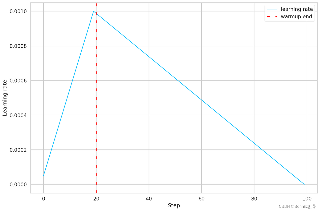

训练步骤的线性学习率调度

我们模拟 100 个训练步骤，并告诉调度程序在前 20 个进行预热。学习率在预热期间增长到初始固定值 0.001，然后（线性）下降到 0。

要使用调度程序，我们需要计算训练和热身步骤的数量。每个时期的训练步数等于number of training examples / batch size。总训练步数为training steps per epoch * number of epochs：

steps_per_epoch=len(train_df) // BATCH_SIZE
total_training_steps = steps_per_epoch * N_EPOCHS

我们将使用五分之一的训练步骤进行热身：

warmup_steps = total_training_steps // 5
warmup_steps, total_training_steps

(5070, 25350)

我们现在可以创建模型的实例：

model = ToxicCommentTagger(
  n_classes=len(LABEL_COLUMNS),
  n_warmup_steps=warmup_steps,
  n_training_steps=total_training_steps
)

评估

多标签分类归结为对每个标签/标记进行二进制分类。

我们将使用二进制交叉熵来衡量每个标签的错误。PyTorch 有BCELoss，我们将把它与一个 sigmoid 函数结合起来（就像我们在模型实现中所做的那样）。让我们看一个例子：

criterion = nn.BCELoss()

prediction = torch.FloatTensor(
  [10.95873564, 1.07321467, 1.58524066, 0.03839076, 15.72987556, 1.09513213]
)
labels = torch.FloatTensor(
  [1., 0., 0., 0., 1., 0.]
)

torch.sigmoid(prediction)

tensor([1.0000, 0.7452, 0.8299, 0.5096, 1.0000, 0.7493])

criterion(torch.sigmoid(prediction), labels)

tensor(0.8725)

我们可以使用相同的方法来计算预测的损失：

_, predictions = model(sample_batch["input_ids"], sample_batch["attention_mask"])
predictions

tensor([[0.3963, 0.6318, 0.6543, 0.5179, 0.4099, 0.4998],
[0.4008, 0.6165, 0.6733, 0.5460, 0.4378, 0.5083],
[0.3877, 0.6185, 0.6830, 0.5238, 0.4326, 0.5138],
[0.3910, 0.6206, 0.6658, 0.5431, 0.4396, 0.5002],
[0.3792, 0.6241, 0.6508, 0.5347, 0.4374, 0.5110],
[0.4069, 0.6106, 0.7019, 0.5484, 0.4450, 0.4995],
[0.3861, 0.6135, 0.6867, 0.5179, 0.4525, 0.5188],
[0.3819, 0.6081, 0.6821, 0.5227, 0.4419, 0.5246]],
grad_fn=<SigmoidBackward>)

criterion(predictions, sample_batch["labels"])

tensor(0.8056, grad_fn=<BinaryCrossEntropyBackward>)

ROC 曲线

我们将要使用的另一个指标是每个标签的接受者操作特征 (ROC) 下的面积。ROC 是通过绘制真阳性率 (TPR) 与假阳性率 (FPR) 来创建的：

TPR=TP/(TP+FN)

FPR=FP/(FP+TN)

from sklearn import metrics

fpr = [0.        , 0.        , 0.        , 0.02857143, 0.02857143,
       0.11428571, 0.11428571, 0.2       , 0.4       , 1.        ]

tpr = [0.        , 0.01265823, 0.67202532, 0.76202532, 0.91468354,
       0.97468354, 0.98734177, 0.98734177, 1.        , 1.        ]

_, ax = plt.subplots()
ax.plot(fpr, tpr, label="ROC")
ax.plot([0.05, 0.95], [0.05, 0.95], transform=ax.transAxes, label="Random classifier", color="red")
ax.legend(loc=4)
ax.set_xlabel("False positive rate")
ax.set_ylabel("True positive rate")
ax.set_title("Example ROC curve")
plt.show();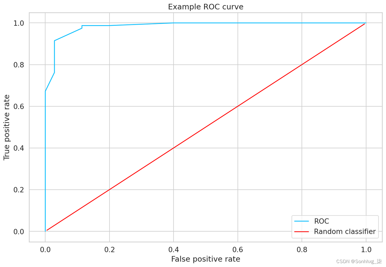

训练分类器与随机分类器的示例 ROC 值

训练

PyTorch Lightning 的美妙之处在于您可以构建您喜欢的标准管道并训练（几乎？）您可能想象的每个模型。我更喜欢使用至少 3 个组件。

保存最佳模型的检查点（基于验证损失）：

checkpoint_callback = ModelCheckpoint(
  dirpath="checkpoints",
  filename="best-checkpoint",
  save_top_k=1,
  verbose=True,
  monitor="val_loss",
  mode="min"
)

在 TensorBoard 中记录进度：

logger = TensorBoardLogger("lightning_logs", name="toxic-comments")

当损失在过去 2 个时期内没有改善时会触发提前停止（在实际项目中进行训练时，您可能想删除/重新考虑这一点）：

early_stopping_callback = EarlyStopping(monitor='val_loss', patience=2)

我们可以开始训练过程：

trainer = pl.Trainer(
  logger=logger,
  checkpoint_callback=checkpoint_callback,
  callbacks=[early_stopping_callback],
  max_epochs=N_EPOCHS,
  gpus=1,
  progress_bar_refresh_rate=30
)

GPU available: True, used: True
TPU available: False, using: 0 TPU cores

trainer.fit(model, data_module)

LOCAL_RANK: 0 - CUDA_VISIBLE_DEVICES: [0]
| Name | Type | Params
-----------------------------------------
| bert | BertModel | 108 M
| classifier | Linear | 4.6 K
| criterion | BCELoss | 0
-----------------------------------------
108 M Trainable params
0 Non-trainable params
108 M Total params
433.260 Total estimated model params size (MB)
Epoch 0, global step 2535: val_loss reached 0.05723 (best 0.05723), saving model to "/content/checkpoints/best-checkpoint.ckpt" as top 1

Epoch 1, global step 5071: val_loss reached 0.04705 (best 0.04705), saving model to "/content/checkpoints/best-checkpoint.ckpt" as top 1

Epoch 2, step 7607: val_loss was not in top 1

Epoch 3, step 10143: val_loss was not in top 1

该模型改进了（仅）2 个时期。我们必须对其进行评估，看看它是否有任何好处。让我们仔细检查验证损失：

trainer.test()

LOCAL_RANK: 0 - CUDA_VISIBLE_DEVICES: [0]

--------------------------------------------------------------------------------DATALOADER:0 TEST RESULTS
{'test_loss': 0.04704693332314491}
--------------------------------------------------------------------------------[{'test_loss': 0.04704693332314491}]

预测

我喜欢在训练完成后查看一小部分预测样本。这建立了关于预测质量的直觉（定性评估）。

让我们加载模型的最佳版本（根据验证损失）：

trained_model = ToxicCommentTagger.load_from_checkpoint(
  trainer.checkpoint_callback.best_model_path,
  n_classes=len(LABEL_COLUMNS)
)

trained_model.eval()
trained_model.freeze()

我们将我们的模型置于“评估”模式，我们准备好做出一些预测。这是对示例（完全虚构的）评论的预测：

test_comment = "Hi, I'm Meredith and I'm an alch... good at supplier relations"

encoding = tokenizer.encode_plus(
  test_comment,
  add_special_tokens=True,
  max_length=512,
  return_token_type_ids=False,
  padding="max_length",
  return_attention_mask=True,
  return_tensors='pt',
)

_, test_prediction = trained_model(encoding["input_ids"], encoding["attention_mask"])
test_prediction = test_prediction.flatten().numpy()

for label, prediction in zip(LABEL_COLUMNS, test_prediction):
  print(f"{label}: {prediction}")

toxic: 0.02174694836139679
severe_toxic: 0.0013127995189279318
obscene: 0.0035953170154243708
threat: 0.0015959267038851976
insult: 0.003400973277166486
identity_hate: 0.003609051927924156

看起来不错。这个很干净。我们将通过阈值 (0.5) 来减少预测的噪音。我们将只采用高于（或等于）阈值的标签预测。让我们尝试一些有毒的东西：

THRESHOLD = 0.5

test_comment = "You are such a loser! You'll regret everything you've done to me!"
encoding = tokenizer.encode_plus(
  test_comment,
  add_special_tokens=True,
  max_length=512,
  return_token_type_ids=False,
  padding="max_length",
  return_attention_mask=True,
  return_tensors='pt',
)

_, test_prediction = trained_model(encoding["input_ids"], encoding["attention_mask"])
test_prediction = test_prediction.flatten().numpy()

for label, prediction in zip(LABEL_COLUMNS, test_prediction):
  if prediction < THRESHOLD:
    continue
  print(f"{label}: {prediction}")

toxic: 0.9569520354270935
insult: 0.7289626002311707

我绝对同意这些标签。看起来我们的模型在这两个例子上做了一些合理的事情。

评估

让我们更全面地了解我们模型的性能。我们将从验证集中的所有预测和标签开始：

device = torch.device('cuda' if torch.cuda.is_available() else 'cpu')
trained_model = trained_model.to(device)

val_dataset = ToxicCommentsDataset(
  val_df,
  tokenizer,
  max_token_len=MAX_TOKEN_COUNT
)

predictions = []
labels = []

for item in tqdm(val_dataset):
  _, prediction = trained_model(
    item["input_ids"].unsqueeze(dim=0).to(device),
    item["attention_mask"].unsqueeze(dim=0).to(device)
  )
  predictions.append(prediction.flatten())
  labels.append(item["labels"].int())

predictions = torch.stack(predictions).detach().cpu()
labels = torch.stack(labels).detach().cpu()

一个简单的指标是模型的准确性：

accuracy(predictions, labels, threshold=THRESHOLD)

tensor(0.9813)

这很好，但你应该对这个结果持保留态度。我们有一个非常不平衡的数据集。让我们检查每个标签的 ROC：

print("AUROC per tag")
for i, name in enumerate(LABEL_COLUMNS):
  tag_auroc = auroc(predictions[:, i], labels[:, i], pos_label=1)
  print(f"{name}: {tag_auroc}")

AUROC per tag
toxic: 0.985722541809082
severe_toxic: 0.990084171295166
obscene: 0.995059609413147
threat: 0.9909615516662598
insult: 0.9884428977966309
identity_hate: 0.9890572428703308

非常好的结果，但就在我们去聚会之前，让我们检查一下每个班级的分类报告。为了使这项工作有效，我们必须对预测应用阈值：

y_pred = predictions.numpy()
y_true = labels.numpy()

upper, lower = 1, 0

y_pred = np.where(y_pred > THRESHOLD, upper, lower)

print(classification_report(
  y_true,
  y_pred,
  target_names=LABEL_COLUMNS,
  zero_division=0
))

precision    recall  f1-score   support
            toxic       0.68      0.91      0.78       748
     severe_toxic       0.53      0.30      0.38        80
          obscene       0.79      0.87      0.83       421
           threat       0.23      0.38      0.29        13
           insult       0.79      0.70      0.74       410
    identity_hate       0.59      0.62      0.60        71
        micro avg       0.72      0.81      0.76      1743
        macro avg       0.60      0.63      0.60      1743
     weighted avg       0.72      0.81      0.75      1743
      samples avg       0.08      0.08      0.08      1743

这让我们对整体表现有了更真实的了解。该模型在标签上出错会导致少量示例。你能为这个做什么？