目标：理解slam的框架以及它的理论知识。供以后自己查阅。

这一章主要非常重要，也是理解后续优化的基础，它是将旋转矩阵和平移向量，转化为李代数的形式进行优化，因为它有很多好处。好处如下：

意思就是采用$R,t$的矩阵表达形式，有冗余。因为旋转向量内部的$R$的９个变量之间有约束，不利于优化。它可以转化为可以用三个无关变量表示的，转化为无约束的能量函数。这也是下面说的李代数。

1) 李代数：

这一章需要介绍一个基本的代数结构(大学的线性代数和离散数学里面有这方面的概念介绍)：群
集合：$A$, 运算为$\cdot$, 如果当运算满足以下性质时，称$(A,\cdot )$为群。
性质：
1:封闭性：$\forall a_1,a_2\in A,a_1\cdot a_2\in A$
2:结合律：$\forall a_1,a_2,a_3\in A,(a_1\cdot a_2)\cdot a_3=a_1\cdot (a_2\cdot a_3)$
3:幺元：$\exists a_0\in A,s.t.\forall a\in A,a_0\cdot a=a\cdot a_0=a$
4:逆：$\forall a\in A,\exists a^{-1}\in A,s.t.a\cdot a^{-1}=a_0$

上一章节讲了旋转矩阵$R$和平移向量$t$，总结如下它们都满足群的性质，且是一些特殊群。是群的一部分，如下：

三维旋转矩阵构成特殊正交群$SO(3)$:

$$SO(3)=\left\{\begin{array}{c}\mathbf{R}\in R^{3\times 3}|\mathbf{R}{\mathbf{R}}^T=I,det(\mathbf{R})=1\end{array}\right\}(1)$$

三维变换矩阵构成特殊特殊欧式群
$$SE(3)=\left\{\begin{array}{c}\mathbf{T}=\left[\begin{array}{cc}\mathbf{R}& t\\ 0^T& 1\end{array}\right]\in R^{4\times 4}|\mathbf{R}\in SO(3),T\in R^3\end{array}\right\}(2)$$

可以验证：
旋转矩阵集合和矩阵乘法构成群。
变换矩阵和矩阵乘法构成群
可以统称旋转矩阵群，和变换矩阵群。
其它常见的群。
（私下可以验证上述４个性质）
在ＳＬＡＭ中，$SO(2),SO(3);SE(2),SE(3)$非常常见的群。
群论是一门课题，一般理论数学比较多。后续介绍其中的李群
李群(Lie Group)
具有连续的性质的群。
既有群也是流形
因为刚体运动中一般为空间连续运动，可以看到$SO(3),SE(3)$都是李群（连续性）。
群中的性质，只有乘法，没有加法，这个限制了很多运算。如求导和求极限。

为了解决没有加法的问题，引出李代数的概念。
李代数：和李群对应的结构，位于向量空间。是李群单位处的正切空间。(见下图使用小写的$so(3)$表示)

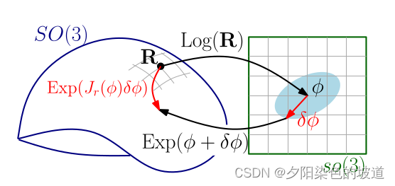
后面介绍上述图像表示的意思为啥成立。
引出李代数：
任意的旋转矩阵$R$，满足：
$$R{R}^T=I(3)$$

考虑到$R$随着时间的变化，有：
$$R(t)R(t{)}^T=I$$

两侧对时间求导：
$$\begin{gathered} \dot{R}(t)R(t{)}^T+R(t)\dot{R}(t{)}^T=0 \\ =>\dot{R}(t)R(t{)}^T=-(\dot{R}(t)R(t{)}^T{)}^T(4) \end{gathered}$$

通过上述的公式$(4)$得到$\dot{R}(t)R(t{)}^T$是反对称矩阵。可以写成一个符号($a$为向量；$A$是矩阵)：
$$a^{\wedge }=A=\left[\begin{array}{ccc}0& -a_3& a_2\\ a_3& 0& -a_1\\ -a_2& a_1& 0\end{array}\right];A^{\vee }=a$$

替换符号反对称矩阵（为了简便看）：
$$\dot{R}(t)R(t{)}^T={\varphi }^{\wedge }(5)$$

将公式$(5)$左右乘$R(t)$可以得到如下：

$$\dot{R}(t)={\varphi }^{\wedge }R(t)(6)$$

可以看到对$R(t)$求导其实是左乘一个反对称矩阵。

公式$(6)$是一个非常重要的公式，也是后续计算的基础。因为有泰勒展开这个法宝。假设在$t_0$时刻泰勒展开，得到如下：
$$R(t)=R(t_0)+\dot{R}(t_0)(t-t_0)+\cdot \cdot \cdot$$

一般情况下是求得一节求导比较多，省略后面的高阶项。
$$\begin{gathered} R(t)=R(t_0)+\dot{R}(t_0)(t-t_0) \\ ＝R(t_0)+\varphi (t_0{)}^{\wedge }(t)(7) \end{gathered}$$
可以看到${\varphi }^{\wedge }$它就是在$R(t)$的正切空间上(见上图)。
因此在连续的空间中，$t_0$附近，$\varphi$不变情况下，有微分方程：

$$\dot{R}(t)=\varphi (t_0{)}^{\wedge }R(t)=\varphi (0{)}^{\wedge }R(t)(8)$$

如果$R(0)=I$，代入到公式$(8)$,解方程得到（因为$exp(x)=exp(x)$，其它为常数项，很容易得到）：

$$R(t)=exp({\varphi }_0^{\wedge }t)(9)$$

上面的公式得到对于任意的$t$,可以找到对应的关系$R$和$\varphi$对应关系。这里称$\varphi$为李代数$so(3)$。

它也有很多性质和定义：
李代数由一个集合$V$,一个数域$F$和一个二元运算$[,]$组成，同事满足下列性质，称为$(V,F,[,])$为李代数，即为$G$。
1:封闭性：$\forall X,Y\in V,[X,Y]\in V$
2:双线性： $\forall X,Y,Z\in V;a,b\in F$,有：$[aX+bY,Z]=a[X,Y]+b[Y,Z],[Z,aX+bY]=a[Z,X]+b[Z,Y]$
3:自反性：$\forall X\in V,[X,X]=0$
4:雅克比等价：$\forall X,Y,Z\in V,[X,[Y,Z]]+[Z,[Y,Z]]+[Y,[Z,X]]=0$

其中二元运算$[,]被称为李括号$
在日常的SLAM中，发现三维空间向量+差积的运算构成李代数。表示如下：
$$so(3)=\left\{\begin{array}{c}\varphi \in R^3,\Phi ={\varphi }^{\wedge }\in R^{3\times 3}\end{array}\right\}(10)$$

其中
$$\Phi ={\varphi }^{\wedge }=\left[\begin{array}{ccc}0& -{\varphi }_3& {\varphi }_2\\ {\varphi }_3& 0& -{\varphi }_1\\ -{\varphi }_2& {\varphi }_1& 0\end{array}\right]\in R^{3\times 3}$$

同理，对于李代数$se(3)$:

$$se(3)=\left\{\begin{array}{c}\xi =\left[\begin{array}{c}\rho \\ \varphi \end{array}\right]\in R^6,\rho \in R^3,\varphi \in so(3),{\xi }^{\wedge }=\left[\begin{array}{cc}{\varphi }^{\wedge }& \rho \\ 0^T& 0\end{array}\right]\in R^{4\times 4}\end{array}\right\}(11)$$

其中$se(3)$是由三个平移分量和三个旋转分量组成。
旋转和$so(3)$相同
平移是一个普通的向量
这个上尖尖不再是反对称矩阵。
$${\xi }^{\wedge }=\left[\begin{array}{cc}{\varphi }^{\wedge }& \rho \\ 0^T& 0\end{array}\right]\in R^{4\times 4}(12)$$

上面的公式是基本的概念，是后续优化的基础。

下面介绍优化的formulation

2)指数映射和对数映射

指数映射反映从李代数到李群的对应关系：
$$R=exp({\varphi }^{\wedge })$$

其中${\varphi }^{\wedge }$为一个矩阵，怎么定义矩阵的运算？直接用Taylor展开。
$$exp({\varphi }^{\wedge })=\sum _{n=0}^{\infty }\frac{1}{n!}({\varphi }^{\wedge }{)}^n$$

需要化简上面的泰勒公式（因为${\varphi }^{\wedge }$是矩阵）。
利用$\varphi$向量的一些性质来处理${\varphi }^{\wedge }$矩阵。
分开$\varphi$向量为方向和模长：$\varphi =\theta a$
因为$a$为单位向量，所以有以下性质：
$$\begin{gathered} a^{\wedge }{a}^{\wedge }=a{a}^T-I(13) \\ {a}^{\wedge }{a}^{\wedge }{a}^{\wedge }=-a^{\wedge }(14) \end{gathered}$$
利用上述的$(13),(14)$公式化解上面的泰勒公式。
泰勒展开后得到：
$$\begin{gathered} exp({\varphi }^{\wedge })=exp(\theta a^{\wedge })=\sum _{n=0}^{\infty }\frac{1}{n!}(\theta a^{\wedge }{)}^n \\ =I+\theta a^{\wedge }+\frac{1}{2!}{\theta }^2(a^{\wedge }{a}^{\wedge })+\frac{1}{3!}{\theta }^3(a^{\wedge }{a}^{\wedge }{a}^{\wedge })+... \\ =a{a}^T-a^{\wedge }{a}^{\wedge }+\theta a^{\wedge }+\frac{1}{2!}{\theta }^2(a^{\wedge }{a}^{\wedge })-\frac{1}{3!}{\theta }^3(a^{\wedge })+... \\ =a{a}^T+(\theta -\frac{1}{3!}{\theta }^3+\frac{1}{5!}{\theta }^5-...)a^{\wedge }-(1-\frac{1}{2!}{\theta }^2+\frac{1}{4!}{\theta }^4-...)a^{\wedge }{a}^{\wedge } \\ =a^{\wedge }{a}^{\wedge }+I+sin\theta a^{\wedge }-cos\theta a^{\wedge }{a}^{\wedge } \\ =(1-cos\theta )a^{\wedge }{a}^{\wedge }+I+sin\theta a^{\wedge } \\ =cos\theta I+(1-cos\theta )a{a}^T+sin\theta a^{\wedge }(15) \end{gathered}$$

最后得到如下：
$$exp(\theta a^{\wedge })=cos\theta I+(1-cos\theta )a{a}^T+sin\theta a^{\wedge }(16)$$

上述就是罗德里公式，可以看到$so(3)$的物理意义为旋转向量。
$$\varphi =In(R{)}^{\vee }=(\sum _{n=0}^{\infty }\frac{(-1{)}^n}{n+1}(R-I{)}^{n+1}{)}^{\vee }(17)$$

上面就介绍了从$SO(3)$到$so(3)$的对应关系。