【池化方法】多示例学习池化（MIL pooling）公式与代码

news2025/11/4 12:20:43

一般的池化方法包括最大池化、平均池化、自适应池化与随机池化，这几天意外看到了多示例学习池化，感觉挺有意思的，记录一下。
论文
代码

1. 多示例学习（Multiple instance learning，MIL）

经典深度学习的数据是一张图一个类别，而多示例学习的数据是一个数据包（bag），一个bag标记一个类别，bag中的每一张图称为一个示例（instance）。形象一点的例子就是，一位患者扫了一次CT，产生了很多张CT切片图像，此时，一张CT切片为一个instance，所有CT切片为一个bag。如果所有的CT切片都检测为没病，那么这位患者正常，否则，这名患者患病。
其基本模式如下图所示：
在这里插入图片描述

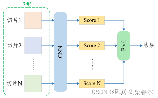
2. MIL pooling

最大池化和平均池化都是不可训练的，设计灵活且自适应的MIL池化可以通过针对任务和数据进行调整，以实现更好的结果。

2.1 注意机制（Attention mechanism）

该方法使用每一个instance低维嵌入的加权平均值，其权重系数通过神经网络学习得到，权重系数之和为1。设 $\left\{ {{h_1}, \ldots ,{h_K}} \right\}$ 为一个bag中的K个嵌入，则：
$\sum\limits_{k = 1}^K {{a_k}{h_k}}}$ ${{a_k} = \frac{{\exp \left\{ {{w^ \top }\tanh (Vh_k^ \top )} \right\}}}{{\sum\limits_{j = 1}^K {\exp \left\{ {{w^ \top }\tanh (Vh_j^ \top )} \right\}} }}}$ 其中 $\in R{^{L \times 1}}}$ , $\in R{^{L \times M}}}$ 为参数，可由全连接层实现。 ${L}$ 为低维嵌入大小， ${M}$ 为中间维度。

2.2 门控注意机制（Gated attention mechanism）

由于 ${\tanh (x)}$ 在 $\in [ - 1,1]}$ 时近似线性，这可能会限制instance之间学习关系的最终表达。作者设计了一种门控机制，即：
${{a_k} = \frac{{\exp \left\{ {{w^ \top }(\tanh (Vh_k^ \top ) \odot sigmoid(Uh_k^ \top ))} \right\}}}{{\sum\limits_{j = 1}^K {\exp \left\{ {{w^ \top }(\tanh (Vh_j^ \top ) \odot sigmoid(Uh_j^ \top ))} \right\}} }}}$ 其中， $\in R{^{L \times M}}}$ 为参数， $\odot }$ 为元素级相乘，门控机制引入了可学习的非线性，潜在地消除了 ${\tanh (x)}$ 中麻烦的线性。

3. MIL pooling的PyTorch代码

import torch
import torch.nn as nn
import torch.nn.functional as F


class Attention(nn.Module):
    def __init__(self):
        super(Attention, self).__init__()
        self.L = 500
        self.D = 128
        self.K = 1

        self.feature_extractor_part1 = nn.Sequential(
            nn.Conv2d(1, 20, kernel_size=5),
            nn.ReLU(),
            nn.MaxPool2d(2, stride=2),
            nn.Conv2d(20, 50, kernel_size=5),
            nn.ReLU(),
            nn.MaxPool2d(2, stride=2)
        )

        self.feature_extractor_part2 = nn.Sequential(
            nn.Linear(50 * 4 * 4, self.L),
            nn.ReLU(),
        )
        # w 和 V 由两个线性层实现
        self.attention = nn.Sequential(
            nn.Linear(self.L, self.D),
            nn.Tanh(),
            nn.Linear(self.D, self.K)
        )

        self.classifier = nn.Sequential(
            nn.Linear(self.L*self.K, 1),
            nn.Sigmoid()
        )

    def forward(self, x):
        # 设输入张量大小为[20, 1, 30, 30]，即有20个instance
        x = x.squeeze(0)   # [20, 1, 30, 30]
       
        H = self.feature_extractor_part1(x)  # [20, 50, 4, 4] 特征提取下采样
        
        H = H.view(-1, 50 * 4 * 4)   # [20, 800] 通道合并
        
        H = self.feature_extractor_part2(H)  # NxL  [20, 500] 低维嵌入
        
        A = self.attention(H)  # NxK  [20, 1] 计算ak
       
        A = torch.transpose(A, 1, 0)  # KxN  [1, 20] 每个instance一个权重
        
        A = F.softmax(A, dim=1)  # softmax over N  [1, 20] softmax使权重之和为1

        M = torch.mm(A, H)  # KxL  [1, 500] 计算ak乘以hk

        Y_prob = self.classifier(M)  # [1, 1] 分类器输出概率
        
        Y_hat = torch.ge(Y_prob, 0.5).float()  # [1, 1] 大于0.5为1

        return Y_prob, Y_hat, A


class GatedAttention(nn.Module):
    def __init__(self):
        super(GatedAttention, self).__init__()
        self.L = 500
        self.D = 128
        self.K = 1

        self.feature_extractor_part1 = nn.Sequential(
            nn.Conv2d(1, 20, kernel_size=5),
            nn.ReLU(),
            nn.MaxPool2d(2, stride=2),
            nn.Conv2d(20, 50, kernel_size=5),
            nn.ReLU(),
            nn.MaxPool2d(2, stride=2)
        )

        self.feature_extractor_part2 = nn.Sequential(
            nn.Linear(50 * 4 * 4, self.L),
            nn.ReLU(),
        )

        self.attention_V = nn.Sequential(
            nn.Linear(self.L, self.D),
            nn.Tanh()
        )

        self.attention_U = nn.Sequential(
            nn.Linear(self.L, self.D),
            nn.Sigmoid()
        )
       
        self.attention_weights = nn.Linear(self.D, self.K)   # w

        self.classifier = nn.Sequential(
            nn.Linear(self.L*self.K, 1),
            nn.Sigmoid()
        )

    def forward(self, x):
        x = x.squeeze(0)

        H = self.feature_extractor_part1(x)
        H = H.view(-1, 50 * 4 * 4)
        H = self.feature_extractor_part2(H)  # NxL

        A_V = self.attention_V(H)  # NxD tanh
        A_U = self.attention_U(H)  # NxD Sigmoid
        A = self.attention_weights(A_V * A_U) # element wise multiplication # NxK
        A = torch.transpose(A, 1, 0)  # KxN
        A = F.softmax(A, dim=1)  # softmax over N

        M = torch.mm(A, H)  # KxL

        Y_prob = self.classifier(M)
        Y_hat = torch.ge(Y_prob, 0.5).float()

        return Y_prob, Y_hat, A