第四章.神经网络
4.3 BP神经网络
BP神经网络(误差反向传播算法)是整个人工神经网络体系中的精华,广泛应用于分类识别,逼近,回归,压缩等领域,在实际应用中,大约80%的神经网络模型都采用BP网络或BP网络的变化形式。
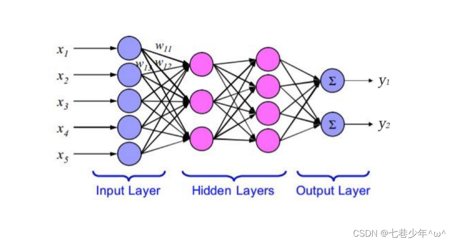
1.网络结构
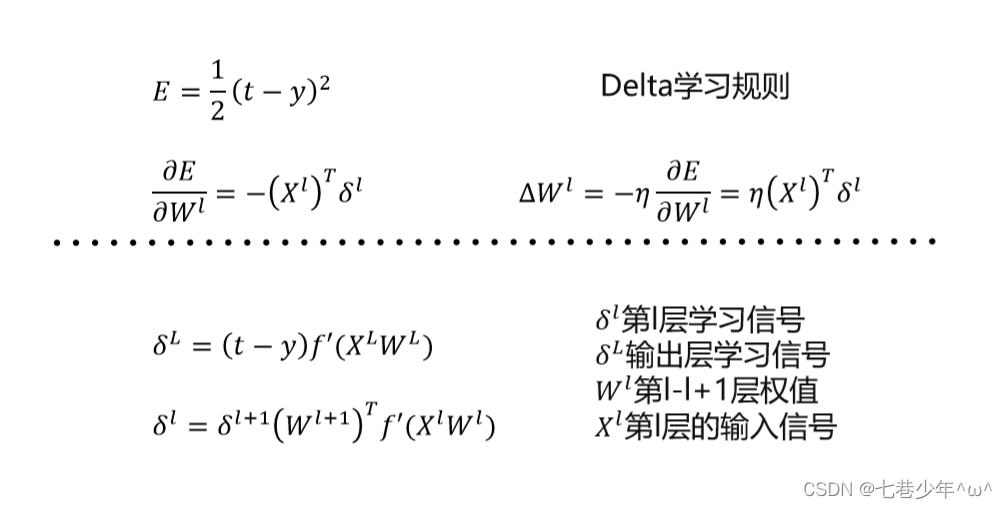
2.公式
3.激活函数
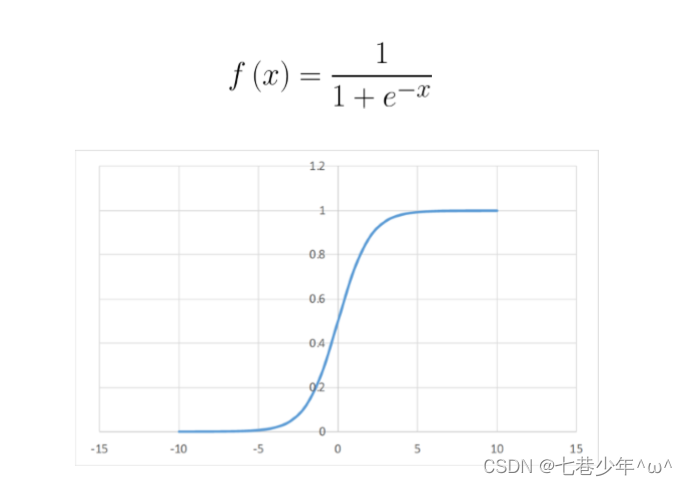
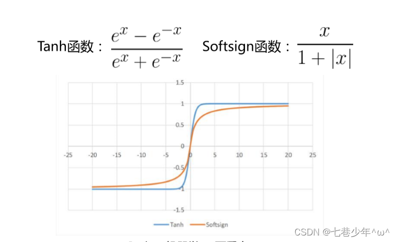
这三个激活函数(Sigmoid,Tanh,Softsign)都存在一个问题,这几个函数的导数几乎都是小于1的,卷积层最多可以有5,6层,层数太多可能无法正常学习。
1).Sigmoid函数:
2).Tanh函数和Softsign函数:
- 图像
- 权重初始值的设置方式:
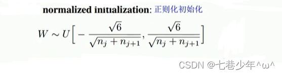
参数说明
①.nj:上一层神经元的个数
②.nj+1:下一层神经元的个数
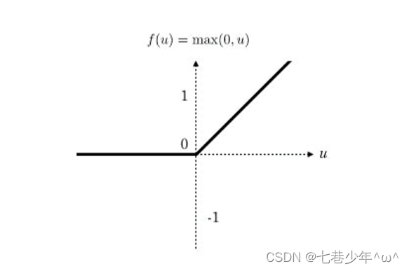
3).ReLu函数:
4.BP网络示例1: 解决异或问题
1).代码:
import numpy as np
import matplotlib.pyplot as plt


# 激活函数:sigmoid
# 正向传播
def sigmoid(x):
    return 1 / (1 + np.exp(-x))


# 反向传播
def dsigmoid(x):
    return x * (1 - x)


def update():
    global X, T, W, V, lr
    L1 = sigmoid(np.dot(X, V))
    L2 = sigmoid(np.dot(L1, W))

    L2_delta = (T.T - L2) * dsigmoid(L2)
    L1_delta = L2_delta.dot(W.T) * dsigmoid(L1)

    W_C = lr * L1.T.dot(L2_delta)
    V_C = lr * X.T.dot(L1_delta)

    W += W_C
    V += V_C


# 判断输出值的是否大于0.5.sigmoid函数是关于(x, y)=(0, 0.5)对称的S型曲线
def judge(x):
    if x > 0.5:
        return 1
    else:
        return 0


# 输入数据
X = np.array([[1, 0, 0], [1, 0, 1], [1, 1, 0], [1, 1, 1]])

# 标签
T = np.array([[0, 1, 1, 0]])

# 权重初始值
V = np.random.random([3, 4]) * 2 - 1
W = np.random.random([4, 1]) * 2 - 1

# 超参数设置
lr = 0.11
epoch = 20000

error = []
for i in range(epoch):
    update()
    if i % 500 == 0:
        L1 = sigmoid(np.dot(X, V))
        L2 = sigmoid(np.dot(L1, W))
        error.append(np.mean(np.abs(T.T - L2)))

L1 = sigmoid(np.dot(X, V))
L2 = sigmoid(np.dot(L1, W))

for i in map(judge, L2):
    print(i)

plt.figure(figsize=(6, 4))
x = np.arange(len(error))
plt.plot(x, error, 'r')
plt.xlabel('epoch')
plt.ylabel('error')
plt.show()
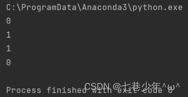
2).结果展示:
5.BP网络示例2: 手写数字识别
1).代码:
import numpy as np
import matplotlib.pyplot as plt
from sklearn.datasets import load_digits
from sklearn.preprocessing import LabelBinarizer
from sklearn.model_selection import train_test_split
# 激活函数:sigmoid
# 正向传播
def sigmoid(x):
return 1 / (1 + np.exp(-x))
# 反向传播
def dsigmoid(x):
return x * (1 - x)
class NeuralNetwork:
def __init__(self, layers):
# 权值的初始值,范围[-1,1]
self.V = np.random.random((layers[0] + 1, layers[1] + 1)) * 2 - 1
self.W = np.random.random((layers[1] + 1, layers[2])) * 2 - 1
# 推理函数
def predict(self, x):
# 添加偏置
temp = np.ones(x.shape[0] + 1)
temp[0:-1] = x
x = temp
x = np.atleast_2d(x)
L1 = sigmoid(np.dot(x, self.V))
L2 = sigmoid(np.dot(L1, self.W))
return L2
def train(self, X, T, lr, epochs):
# 添加偏置
temp = np.ones([X.shape[0], X.shape[1] + 1])
temp[:, 0:-1] = X
X = temp
for n in range(epochs + 1):
i = np.random.randint(X.shape[0]) # 随机选取一个数据
x = [X[i]]
x = np.atleast_2d(x) # 转为2维数据
L1 = sigmoid(np.dot(x, self.V))
L2 = sigmoid(np.dot(L1, self.W))
L2_detal = (T[i] - L2) * dsigmoid(L2)
L1_detal = L2_detal.dot(self.W.T) * dsigmoid(L1)
W_C = lr * L1.T.dot(L2_detal)
V_C = lr * x.T.dot(L1_detal)
self.W += W_C
self.V += V_C
# 每训练1000次预测一次精度
if n % 1000 == 0:
predictions = []
for j in range(X_test.shape[0]):
output = self.predict(X_test[j])
predictions.append(np.argmax(output))
accuracy = np.mean(np.equal(predictions, T_test))
accuracys.append(accuracy)
print('epoch:', n, 'accuracy:', accuracy)
# 加载数据
digits = load_digits()
# 数据和标签
X = digits.data
T = digits.target
# 输入数据归一化
X = (X - X.min()) / X.max()
# 创建网络[64,100,10]
nm = NeuralNetwork([64, 100, 10])
# 分割数据: 1/4为测试数据,3/4为训练数据
X_train, X_test, T_train, T_test = train_test_split(X, T)
# 标签二值化 0,8,6 0->1000000000 3->0001000000
labels_train = LabelBinarizer().fit_transform(T_train)
print('start:')
accuracys = []
nm.train(X_train, labels_train, lr=0.11, epochs=20000)
print('end')
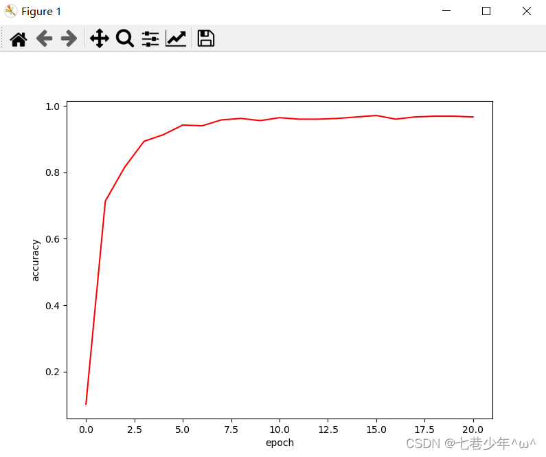
plt.figure(figsize=(8, 6))
x_data = np.arange(len(accuracys))
plt.plot(x_data, accuracys, 'r')
plt.xlabel('epoch')
plt.ylabel('accuracy')
plt.show()
2).结果展示:
6.混淆矩阵
1).示例:
- 假设有一个用来对猫(cats),狗(dogs),兔子(rabbits)进行分类的系统,混淆矩阵就是为了进一步分析性能而对该算法测试结果做出的总结。
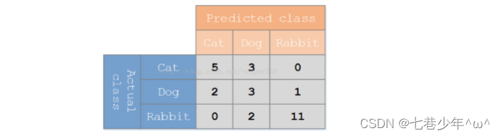
- 在这个混淆矩阵中,实际有8只猫,但是系统将其中的3只预测成了狗,实际6只狗,其中一只被预测成了兔子,两只被预测成了猫。
7.神经网络: sklearn手写数字识别
1).代码:
from sklearn.datasets import load_digits
from sklearn.neural_network import MLPClassifier
from sklearn.model_selection import train_test_split
from sklearn.preprocessing import StandardScaler
from sklearn.metrics import classification_report, confusion_matrix
# 加载数据
digits = load_digits()
# 数据和标签
x_data = digits.data
t_data = digits.target
# 标准化
scaler = StandardScaler()
x_data = scaler.fit_transform(x_data)
x_train, x_test, t_train, t_test = train_test_split(x_data, t_data)
# 创建模型和训练
mlp = MLPClassifier(hidden_layer_sizes=(100, 50), max_iter=1000)
mlp.fit(x_train, t_train)
prediction = mlp.predict(x_test)
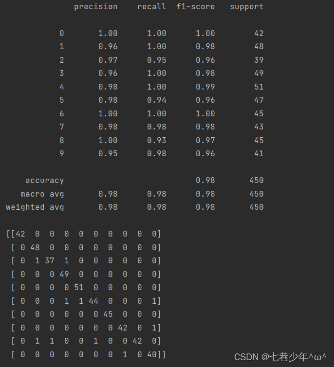
print(classification_report(t_test, prediction))
print(confusion_matrix(t_test, prediction))
2).结果展示:
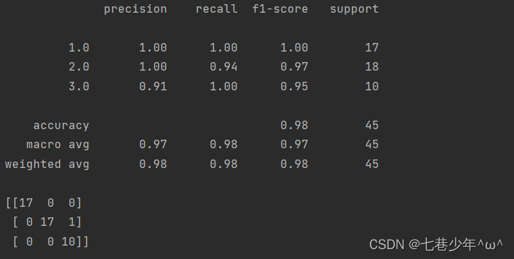
8.神经网络:葡萄酒品质分类
1).示例:
- 我们将使用一个葡萄酒数据集。它具有不同葡萄酒的各 种化学特征,均在意大利同一地区生长,但数据标签分 类为三种不同的品种。我们将尝试建立一个可以根据其 化学特征对葡萄酒品种进行分类的神经网络模型
2).代码:
import numpy as np
from sklearn.model_selection import train_test_split
from sklearn.preprocessing import StandardScaler
from sklearn.neural_network import MLPClassifier
from sklearn.metrics import classification_report, confusion_matrix

# 加载数据
data = np.genfromtxt('D:\\data\\wine_data.csv', delimiter=',')

# 数据和标签
x_data = data[:, 1:]
t_data = data[:, 0]

# 测试数据和训练数据的切分
x_train, x_test, t_train, t_test = train_test_split(x_data, t_data)

# 数据标准化
scaler = StandardScaler()
x_train = scaler.fit_transform(x_train)
x_test = scaler.fit_transform(x_test)

# 创建模型和训练
mlp = MLPClassifier(hidden_layer_sizes=(100, 50), max_iter=1000)
mlp.fit(x_train, t_train)

# 评估
predictions = mlp.predict(x_test)
print(classification_report(t_test, predictions))
print(confusion_matrix(t_test, predictions))
3).结果展示: