三、通道注意力

3.1 通道注意力的定义

# ===================== 新增：通道注意力模块（SE模块） =====================
class ChannelAttention(nn.Module):
    """通道注意力模块(Squeeze-and-Excitation)"""
    def __init__(self, in_channels, reduction_ratio=16):
        """
        参数:
            in_channels: 输入特征图的通道数
            reduction_ratio: 降维比例，用于减少参数量
        """
        super(ChannelAttention, self).__init__()
        
        # 全局平均池化 - 将空间维度压缩为1x1，保留通道信息
        self.avg_pool = nn.AdaptiveAvgPool2d(1)
        
        # 全连接层 + 激活函数，用于学习通道间的依赖关系
        self.fc = nn.Sequential(
            # 降维：压缩通道数，减少计算量
            nn.Linear(in_channels, in_channels // reduction_ratio, bias=False),
            nn.ReLU(inplace=True),
            # 升维：恢复原始通道数
            nn.Linear(in_channels // reduction_ratio, in_channels, bias=False),
            # Sigmoid将输出值归一化到[0,1]，表示通道重要性权重
            nn.Sigmoid()
        )

    def forward(self, x):
        """
        参数:
            x: 输入特征图，形状为 [batch_size, channels, height, width]
        
        返回:
            加权后的特征图，形状不变
        """
        batch_size, channels, height, width = x.size()
        
        # 1. 全局平均池化：[batch_size, channels, height, width] → [batch_size, channels, 1, 1]
        avg_pool_output = self.avg_pool(x)
        
        # 2. 展平为一维向量：[batch_size, channels, 1, 1] → [batch_size, channels]
        avg_pool_output = avg_pool_output.view(batch_size, channels)
        
        # 3. 通过全连接层学习通道权重：[batch_size, channels] → [batch_size, channels]
        channel_weights = self.fc(avg_pool_output)
        
        # 4. 重塑为二维张量：[batch_size, channels] → [batch_size, channels, 1, 1]
        channel_weights = channel_weights.view(batch_size, channels, 1, 1)
        
        # 5. 将权重应用到原始特征图上（逐通道相乘）
        return x * channel_weights  # 输出形状：[batch_size, channels, height, width]

 3.2 模型的重新定义

class CNN(nn.Module):
    def __init__(self):
        super(CNN, self).__init__()  
        
        # ---------------------- 第一个卷积块 ----------------------
        self.conv1 = nn.Conv2d(3, 32, 3, padding=1)
        self.bn1 = nn.BatchNorm2d(32)
        self.relu1 = nn.ReLU()
        # 新增：插入通道注意力模块（SE模块）
        self.ca1 = ChannelAttention(in_channels=32, reduction_ratio=16)  
        self.pool1 = nn.MaxPool2d(2, 2)  
        
        # ---------------------- 第二个卷积块 ----------------------
        self.conv2 = nn.Conv2d(32, 64, 3, padding=1)
        self.bn2 = nn.BatchNorm2d(64)
        self.relu2 = nn.ReLU()
        # 新增：插入通道注意力模块（SE模块）
        self.ca2 = ChannelAttention(in_channels=64, reduction_ratio=16)  
        self.pool2 = nn.MaxPool2d(2)  
        
        # ---------------------- 第三个卷积块 ----------------------
        self.conv3 = nn.Conv2d(64, 128, 3, padding=1)
        self.bn3 = nn.BatchNorm2d(128)
        self.relu3 = nn.ReLU()
        # 新增：插入通道注意力模块（SE模块）
        self.ca3 = ChannelAttention(in_channels=128, reduction_ratio=16)  
        self.pool3 = nn.MaxPool2d(2)  
        
        # ---------------------- 全连接层（分类器） ----------------------
        self.fc1 = nn.Linear(128 * 4 * 4, 512)
        self.dropout = nn.Dropout(p=0.5)
        self.fc2 = nn.Linear(512, 10)

    def forward(self, x):
        # ---------- 卷积块1处理 ----------
        x = self.conv1(x)       
        x = self.bn1(x)         
        x = self.relu1(x)       
        x = self.ca1(x)  # 应用通道注意力
        x = self.pool1(x)       
        
        # ---------- 卷积块2处理 ----------
        x = self.conv2(x)       
        x = self.bn2(x)         
        x = self.relu2(x)       
        x = self.ca2(x)  # 应用通道注意力
        x = self.pool2(x)       
        
        # ---------- 卷积块3处理 ----------
        x = self.conv3(x)       
        x = self.bn3(x)         
        x = self.relu3(x)       
        x = self.ca3(x)  # 应用通道注意力
        x = self.pool3(x)       
        
        # ---------- 展平与全连接层 ----------
        x = x.view(-1, 128 * 4 * 4)  
        x = self.fc1(x)           
        x = self.relu3(x)         
        x = self.dropout(x)       
        x = self.fc2(x)           
        
        return x  

# 重新初始化模型，包含通道注意力模块
model = CNN()
model = model.to(device)  # 将模型移至GPU（如果可用）

criterion = nn.CrossEntropyLoss()  # 交叉熵损失函数
optimizer = optim.Adam(model.parameters(), lr=0.001)  # Adam优化器

# 引入学习率调度器，在训练过程中动态调整学习率--训练初期使用较大的 LR 快速降低损失，训练后期使用较小的 LR 更精细地逼近全局最优解。
# 在每个 epoch 结束后，需要手动调用调度器来更新学习率，可以在训练过程中调用 scheduler.step()
scheduler = optim.lr_scheduler.ReduceLROnPlateau(
    optimizer,        # 指定要控制的优化器（这里是Adam）
    mode='min',       # 监测的指标是"最小化"（如损失函数）
    patience=3,       # 如果连续3个epoch指标没有改善，才降低LR
    factor=0.5        # 降低LR的比例（新LR = 旧LR × 0.5）
)

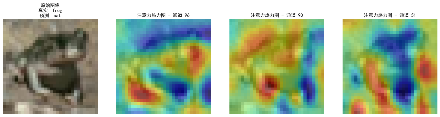
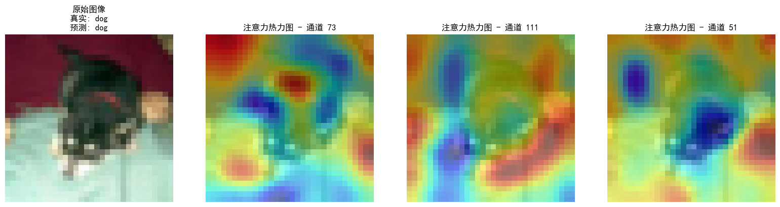
可视化空间注意力热力图

# 可视化空间注意力热力图（显示模型关注的图像区域）
def visualize_attention_map(model, test_loader, device, class_names, num_samples=3):
    """可视化模型的注意力热力图，展示模型关注的图像区域"""
    model.eval()  # 设置为评估模式
    
    with torch.no_grad():
        for i, (images, labels) in enumerate(test_loader):
            if i >= num_samples:  # 只可视化前几个样本
                break
                
            images, labels = images.to(device), labels.to(device)
            
            # 创建一个钩子，捕获中间特征图
            activation_maps = []
            
            def hook(module, input, output):
                activation_maps.append(output.cpu())
            
            # 为最后一个卷积层注册钩子（获取特征图）
            hook_handle = model.conv3.register_forward_hook(hook)
            
            # 前向传播，触发钩子
            outputs = model(images)
            
            # 移除钩子
            hook_handle.remove()
            
            # 获取预测结果
            _, predicted = torch.max(outputs, 1)
            
            # 获取原始图像
            img = images[0].cpu().permute(1, 2, 0).numpy()
            # 反标准化处理
            img = img * np.array([0.2023, 0.1994, 0.2010]).reshape(1, 1, 3) + np.array([0.4914, 0.4822, 0.4465]).reshape(1, 1, 3)
            img = np.clip(img, 0, 1)
            
            # 获取激活图（最后一个卷积层的输出）
            feature_map = activation_maps[0][0].cpu()  # 取第一个样本
            
            # 计算通道注意力权重（使用SE模块的全局平均池化）
            channel_weights = torch.mean(feature_map, dim=(1, 2))  # [C]
            
            # 按权重对通道排序
            sorted_indices = torch.argsort(channel_weights, descending=True)
            
            # 创建子图
            fig, axes = plt.subplots(1, 4, figsize=(16, 4))
            
            # 显示原始图像
            axes[0].imshow(img)
            axes[0].set_title(f'原始图像\n真实: {class_names[labels[0]]}\n预测: {class_names[predicted[0]]}')
            axes[0].axis('off')
            
            # 显示前3个最活跃通道的热力图
            for j in range(3):
                channel_idx = sorted_indices[j]
                # 获取对应通道的特征图
                channel_map = feature_map[channel_idx].numpy()
                # 归一化到[0,1]
                channel_map = (channel_map - channel_map.min()) / (channel_map.max() - channel_map.min() + 1e-8)
                
                # 调整热力图大小以匹配原始图像
                from scipy.ndimage import zoom
                heatmap = zoom(channel_map, (32/feature_map.shape[1], 32/feature_map.shape[2]))
                
                # 显示热力图
                axes[j+1].imshow(img)
                axes[j+1].imshow(heatmap, alpha=0.5, cmap='jet')
                axes[j+1].set_title(f'注意力热力图 - 通道 {channel_idx}')
                axes[j+1].axis('off')
            
            plt.tight_layout()
            plt.show()

# 调用可视化函数
visualize_attention_map(model, test_loader, device, class_names, num_samples=3)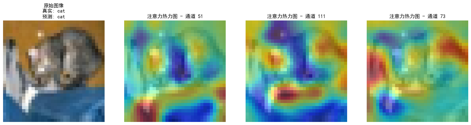

@浙大疏锦行