抑郁症患者数据分析

news2025/6/6 16:32:49

导入数据

import pandas as pd
from pyecharts.charts import *
from pyecharts import options as opts

df=pd.read_csv('YiYuZheng.csv')
df.head(1)

	Patient_name	Label	Date	Title	Communications	Doctor	Hospital	Faculty
0	患者：女 43岁	压抑	05.28	压抑个人情况：去年1月份开始夫妻两地分居，孩子13岁男孩住校，平... 这种情况是否需要去...	115	杨胜文	襄阳市安定医院	心理科

# 查看数据
df.info()

<class 'pandas.core.frame.DataFrame'>
RangeIndex: 8400 entries, 0 to 8399
Data columns (total 8 columns):
 #   Column          Non-Null Count  Dtype 
---  ------          --------------  ----- 
 0   Patient_name    8400 non-null   object
 1   Label           8400 non-null   object
 2   Date            8288 non-null   object
 3   Title           8400 non-null   object
 4   Communications  8400 non-null   int64 
 5   Doctor          8400 non-null   object
 6   Hospital        8400 non-null   object
 7   Faculty         8400 non-null   object
dtypes: int64(1), object(7)
memory usage: 525.1+ KB

从数据反馈结果来看：Date列存在空缺值，并且不是日期类型。

Patient_name列存在信息混合一起情况，需要拆分年龄和性别。

数据预处理

拆分年龄和性别

#获取性别，作为新列
#患者：女 43岁,首先按照空格拆分，结果为[患者：女]\[ ]\[43岁],选取第一个，第二次按照中文冒号拆分，[患者][: ][女]
df['Sex']=df['Patient_name'].map(lambda x:x.split(" ")[0]).map(lambda x:x.split("：")[-1])

#获取年龄，作为新列
#患者：女 43岁,首先按照空格拆分，结果为[患者：女]\[ ]\[43岁],选取第三个，并且去掉“岁”
df['Age']=df['Patient_name'].map(lambda x:x.split(" ")[2][:-1])

df.head()

	Patient_name	Label	Date	Title	Communications	Doctor	Hospital	Faculty	Sex	Age
0	患者：女 43岁	压抑	05.28	压抑个人情况：去年1月份开始夫妻两地分居，孩子13岁男孩住校，平... 这种情况是否需要去...	115	杨胜文	襄阳市安定医院	心理科	女	43
1	患者：女 32岁	生气。心梗。抑郁	05.28	生气。心梗。抑郁郁郁寡欢。被他人语言刺激。卧床不起。没动力。心疼。受伤是什么病。怎么办	12	郭汉法	泰安八十八医院	临床心理科	女	32
2	患者：女 15岁	情绪低落，烦躁抑郁	05.28	情绪低落，烦躁抑郁情绪低落，压抑烦躁，思考能力降低。长时间学习，睡眠时间少。睡... 还有...	2	郭苏皖	南京脑科医院	医学心理科	女	15
3	患者：女 16岁	抑郁	05.28	抑郁前面已简述，2024年夏季中考，本来学习非常好，非常自律，自... 已经服用9个月的艾...	2	刘丽	联勤保障部队第九〇四医院（常州院区）	精神3科（物质依赖科）	女	16
4	患者：女 67岁	焦虑症严重躯干反应、抑郁症	05.28	焦虑症严重躯干反应抑郁症草酸加量以后，还是有比较严重的躯干反应，主要表现为背痛脖...	2	刘晓华	上海市精神卫生中心	精神科	女	67

处理空缺值

df.isnull().sum()

Patient_name        0
Label               0
Date              112
Title               0
Communications      0
Doctor              0
Hospital            0
Faculty             0
Sex                 0
Age                 0
dtype: int64

#因为空缺数据较少，并且不适合使用填充法，故而删除
df.dropna(inplace=True)#在原来的数据上删除

df.info()

<class 'pandas.core.frame.DataFrame'>
Int64Index: 8288 entries, 0 to 8399
Data columns (total 10 columns):
 #   Column          Non-Null Count  Dtype 
---  ------          --------------  ----- 
 0   Patient_name    8288 non-null   object
 1   Label           8288 non-null   object
 2   Date            8288 non-null   object
 3   Title           8288 non-null   object
 4   Communications  8288 non-null   int64 
 5   Doctor          8288 non-null   object
 6   Hospital        8288 non-null   object
 7   Faculty         8288 non-null   object
 8   Sex             8288 non-null   object
 9   Age             8288 non-null   object
dtypes: int64(1), object(9)
memory usage: 712.2+ KB

修改Date列

#df['Date']
#转换成字符串类型
df['Date']=df['Date'].astype(str)

#定义函数，实现date列格式统一：年-月-日
def trans_date(tag):
    if tag.startswith("20"):#查看是否以20开头，即查看是否存在年
        tag=tag.replace(".","-")
    else:
        tag="2025-"+tag.replace(".","-")#否则加上年份
    return tag

df['Date']= df['Date'].map(lambda x:trans_date(x))#调用函数转换格式

#转换成日期类型
df['Date']=pd.to_datetime(df['Date'])

#df.info()

数据可视化分析

from pyecharts.globals import ThemeType #导入主题库

查看患者性别分布情况

#准备数据：按照性别统计个数
data=df['Sex'].value_counts()
#data
x=data.index.tolist()
y=data.tolist()

#绘制饼图
pie=(
    Pie(init_opts=opts.InitOpts(theme=ThemeType.LIGHT))#设置主题
    .add("",
         [list(z) for z in zip(x,y)],#数据需要打包成[(key,value),(key,value),...]
         label_opts=opts.LabelOpts(formatter="{b}:{d}%")#以百分比形式显示标签
        )
    .set_global_opts(title_opts=opts.TitleOpts(title="患者性别分布情况"))
)
pie.render_notebook()

在这里插入图片描述

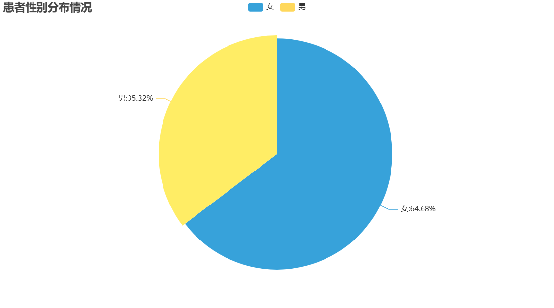
可见：女性抑郁症更为常见。

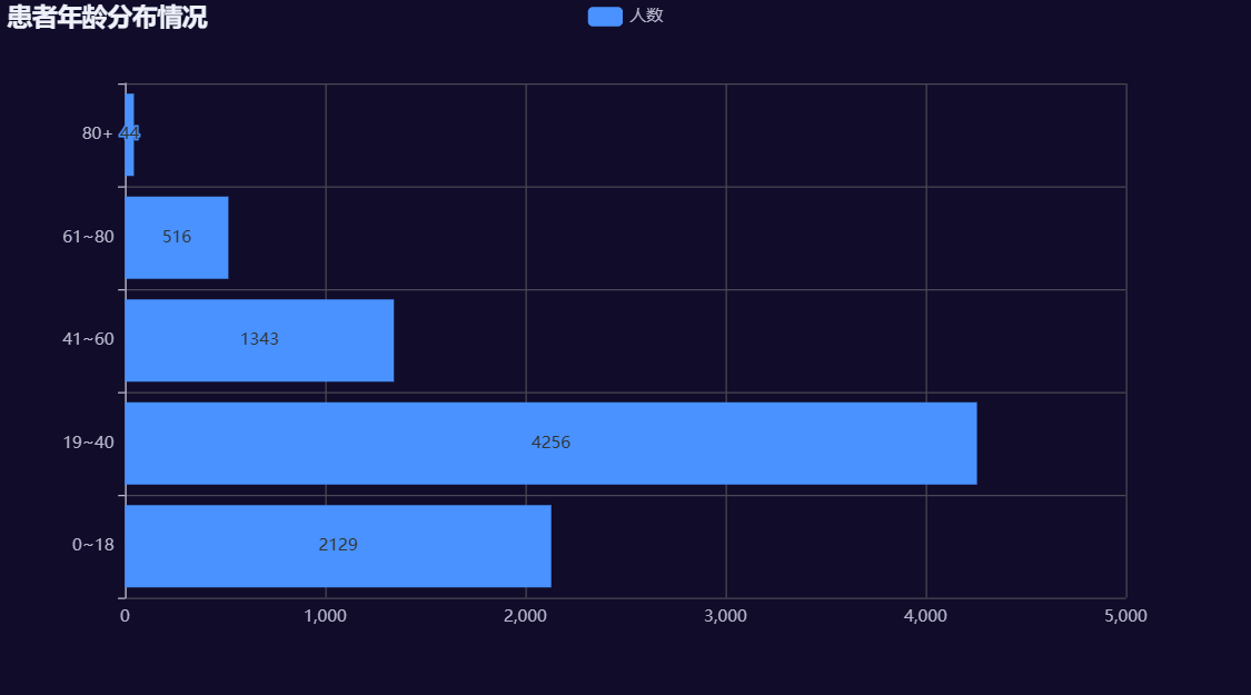
患者年龄分布情况

#数据准备
#1.转换年龄为数值类型
#df['Age']=df['Age'].astype(int)
#因为年龄数据不规范，存在：X岁Y月 形式的数据，再次进行数据处理
df['Age']=df['Age'].map(lambda x:"1" if ("天" in x or "个" in x or "月" in x) else x).astype(int)
#df.info()

#2.年龄分箱
labels=["0~18","19~40","41~60","61~80","80+"]#区间标签
df['age_label']=pd.cut(df['Age'],bins=[0,18,40,60,80,100],labels=labels)#分箱

#3.统计各个年龄区间人数
data=df['age_label'].value_counts().sort_index()#按照索引值排序
#data

x=data.index.tolist()
y=data.tolist()

#画柱状图
bar=(
    Bar(init_opts=opts.InitOpts(theme=ThemeType.DARK))#主题配置
    .add_xaxis(x)
    .add_yaxis("人数",y)
    .set_global_opts(title_opts=opts.TitleOpts(title="患者年龄分布情况"))
    .reversal_axis()
)
bar.render_notebook()

在这里插入图片描述

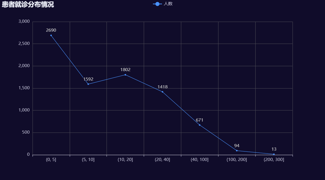
查看患者就诊次数分布

#对就诊次数分箱
bins=[0,5,10,20,40,100,200,300]
df['Communications_count']=pd.cut(df['Communications'],bins=bins)
#按照就诊分箱数据统计数据
data=df['Communications_count'].value_counts().sort_index()#按照索引排序
#data
x=data.index.astype(str).tolist()
y=data.tolist()

#画柱状图
line=(
    Line(init_opts=opts.InitOpts(theme=ThemeType.DARK))#主题配置
    .add_xaxis(x)
    .add_yaxis("人数",y)
    .set_global_opts(title_opts=opts.TitleOpts(title="患者就诊分布情况"),
                    xaxis_opts=opts.AxisOpts(type_='category'),#x轴数据为类别类型
                    yaxis_opts=opts.AxisOpts(type_='value'),)#y轴数据为数值类型
    
)
line.render_notebook()

在这里插入图片描述

    <div id="22f20d64280d408c96ed5b60aa15391a" style="width:900px; height:500px;"></div>

患者标签分布

#pip install jieba

^C
Note: you may need to restart the kernel to use updated packages.

import jieba
from collections import Counter

#定义函数分词
def chinese_word_cut(text):
    seg_list=jieba.cut(text,cut_all=False)
    return [word for word in seg_list if len(word)>1]

#对表格数据进行分词
all_word=[]
for text in df['Title']:
    all_word.extend(chinese_word_cut(text))

#统计词频
word_count=Counter(all_word)
top_words=word_count.most_common(100)#取前100个高频词

data=[(word,count) for word,count in top_words]

w=(
    WordCloud()
    .add("",data)
)
w.render_notebook()

在这里插入图片描述

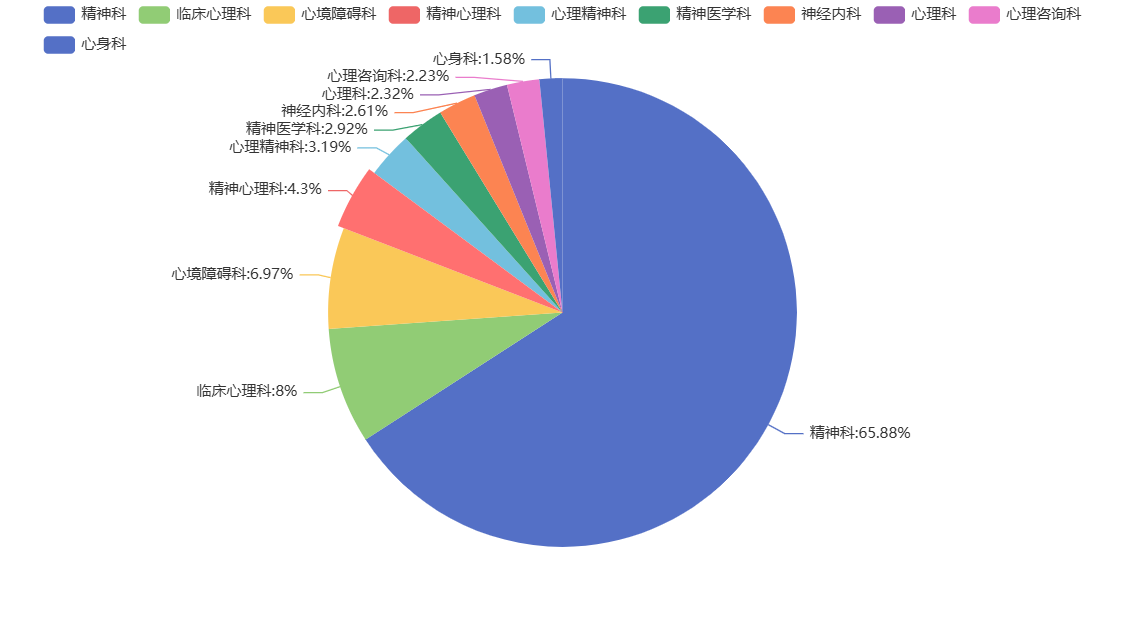
患者就诊的科室分布

data=df['Faculty'].value_counts()[:10] #选取前十科室

pie=(
    Pie()
    .add('',[list(z) for z in zip(data.index.tolist(),data.tolist())],#饼图数据格式[[key1,value1],[key2,value2],...]
        label_opts=opts.LabelOpts(formatter="{b}:{d}%")#标签格式
        )
)
pie.render_notebook()