matplotlib库之核心对象
- Figure
- Figure作用
- Figure常用属性
- Figure常用方法
- Figure对象的创建
- 隐式创建(通过 pyplot)
- 显式创建
- 使用subplots()一次性创建 Figure 和 Axes
- Axes(绘图区)
- Axes创建方式
- Axes基本绘图功能
- Axes绘图的常用参数
- Axes图例参数
- Axes注释参数
- 注释箭头参数(arrowprops)
- 文本框参数(bbox)
- 其它注释参数
- Axes的常用方法
- 基本设置
- 刻度与网格边框
- 图例与注释
- 图形样式
- Axis(坐标轴)
- 获取axis对象
- 刻度位置(Locator)
- 刻度格式(Formatter)
- 隐藏坐标轴或刻度
- 隐藏刻度
- 隐藏边框和设置边框
- 自定义刻度外观
- 共享X轴
- 共享X轴时的legend设置
- 设置对数坐标
- axes和axis的对比
Figure
-🍑 顶级容器,包含所有绘图元素(如 Axes、标题、图例等)。
-🍑 类似于一张空白画布,可以在上面放置多个图表。
Figure作用
-🍑 控制整体图形的尺寸(如figsize=(8, 6))、分辨率(dpi=100)、背景颜色,图名称等。
-🍑 管理多个子图(Axes)的布局。
-🍑 处理图形的保存(如 PNG、PDF)和显示。
-🍑 设置全局标题和其他装饰元素。
Figure常用属性
| 属性 | 说明 | 示例 |
|---|---|---|
| figsize | 图形尺寸(宽 × 高,英寸) | fig = plt.figure(figsize=(8, 6)) |
| dpi | 分辨率(每英寸点数) | fig = plt.figure(dpi=300) |
| facecolor | 背景颜色 | fig = plt.figure(facecolor=‘lightgray’) |
| edgecolor | 边框颜色 | fig = plt.figure(edgecolor=‘black’) |
| linewidth | 边框线宽 | fig = plt.figure(linewidth=2) |
| num | 设置figure的编号或者名称 | fig = plt.figure(num=“figure_168”) |
Figure常用方法
| 方法 | 说明 | 示例 |
|---|---|---|
| add_subplot() | 添加子图(按网格布局) | ax = fig.add_subplot(2, 2, 1)(2×2 网格的第 1 个) |
| add_axes() | 添加自定义位置和大小的子图 | ax = fig.add_axes([0.1, 0.1, 0.8, 0.8])(左下角开始) |
| subplots() | 一次性创建多个子图(返回 Figure 和 Axes 数组) | fig, axes = plt.subplots(2, 2) |
| delaxes() | 删除指定的 Axes | fig.delaxes(ax) |
| suptitle() | 设置全局标题, plt也有此方法 | fig.suptitle(‘Main Title’, fontsize=16) |
| text() | 在任意位置添加文本, plt也有此方法 | fig.text(0.5, 0.95, ‘Annotation’, ha=‘center’) |
| savefig() | 保存图形到文件 | fig.savefig(‘plot.png’, dpi=300, bbox_inches=‘tight’) |
| show() | 显示图形(在交互式环境中) | fig.show() |
| canvas.draw() | 强制重绘图形 | fig.canvas.draw() |
| tight_layout() | 自动调整子图布局,避免元素重叠, plt也有此方法 | fig.tight_layout() |
| subplots_adjust() | 手动调整子图参数(边距、间距等), plt也有此方法 | fig.subplots_adjust(hspace=0.5, wspace=0.3) |
| set_size_inches() | 动态调整图形尺寸 | fig.set_size_inches(12, 8) |
| clear() | 清除图形所有内容,但保留 Figure 对象 | fig.clear() |
| get_children() | 获取所有子元素(包括 Axes、文本等) | children = fig.get_children() |
| number | 获取 Figure 编号(唯一标识) | print(fig.number) |
code:
import matplotlib.pyplot as plt
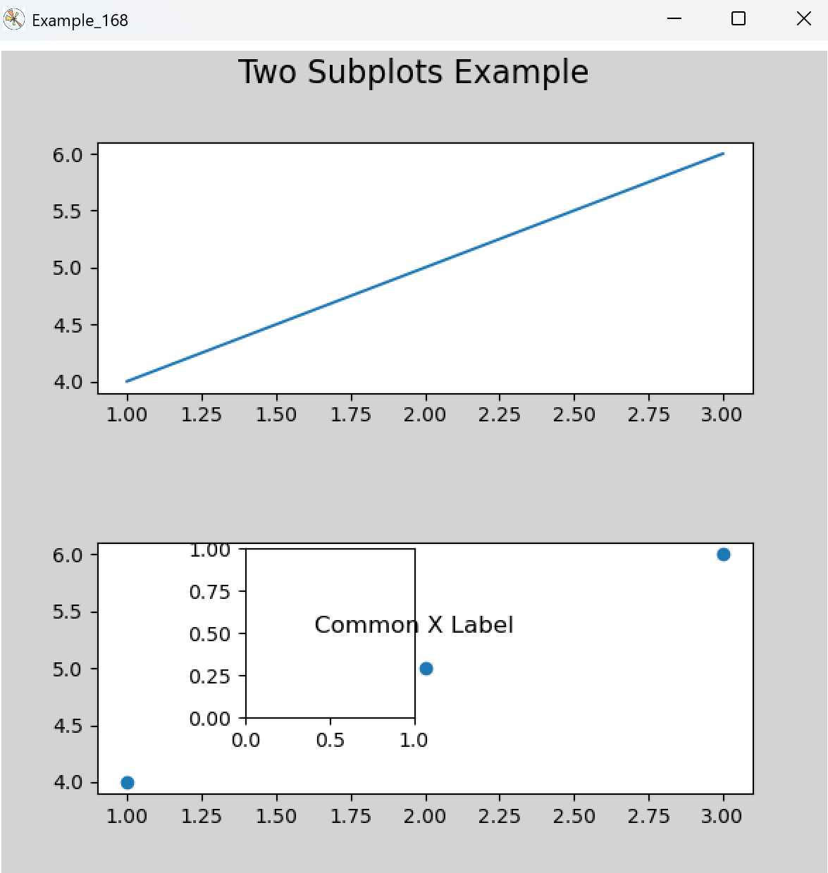
fig = plt.figure(figsize=(6, 6), dpi=100, num="Example_168",linewidth=10, facecolor='lightgray') # 创建Figure对象
ax1 = fig.add_subplot(211) # 2行1列,第1个子图
ax2 = fig.add_subplot(212) # 2行1列,第2个子图
ax3 = fig.add_axes([0.2, 0.2, 0.2, 0.2])
ax1.plot([1, 2, 3], [4, 5, 6]) # 折线图
ax2.scatter([1, 2, 3], [4, 5, 6]) # 散点图
fig.suptitle('Two Subplots Example', fontsize=16) # 设置全局标题
fig.subplots_adjust(hspace=0.6) # 增加子图间距
fig.text(0.5, 0.3, 'Common X Label', ha='center', fontsize=12) # 添加文本注释
fig.savefig('example.png', dpi=300, bbox_inches='tight')
plt.show()
Figure对象的创建
隐式创建(通过 pyplot)
code:
import matplotlib.pyplot as plt

plt.plot([1, 2, 3], [4, 5, 6])  # 自动创建Figure和Axes
fig = plt.gcf()  # 获取当前Figure对象
显式创建
code:

fig = plt.figure(figsize=(10, 5), dpi=100)  # 直接创建Figure
ax = fig.add_subplot(111)  # 添加一个Axes
ax.plot([1, 2, 3], [4, 5, 6])
使用subplots()一次性创建 Figure 和 Axes
code:
fig, axes = plt.subplots(2, 2, figsize=(10, 8))  # 创建2×2网格的子图
axes[0, 0].plot([1, 2])  # 左上角子图
Axes(绘图区)
-🍓 实际的绘图区域,包含具体的数据可视化。
-🍓 绘制具体图表(如折线图、散点图)。
-🍓 设置标题、图例、网格等。
-🍓 管理两个或三个 Axis 对象:X 轴、Y 轴(3D 图还有 Z 轴)。
-🍓 一个Figure可包含多个axes。
Axes创建方式
- 🍌 使用 plt.subplots(),见figure的创建方式。
- 🍌 使用 plt.subplot()。
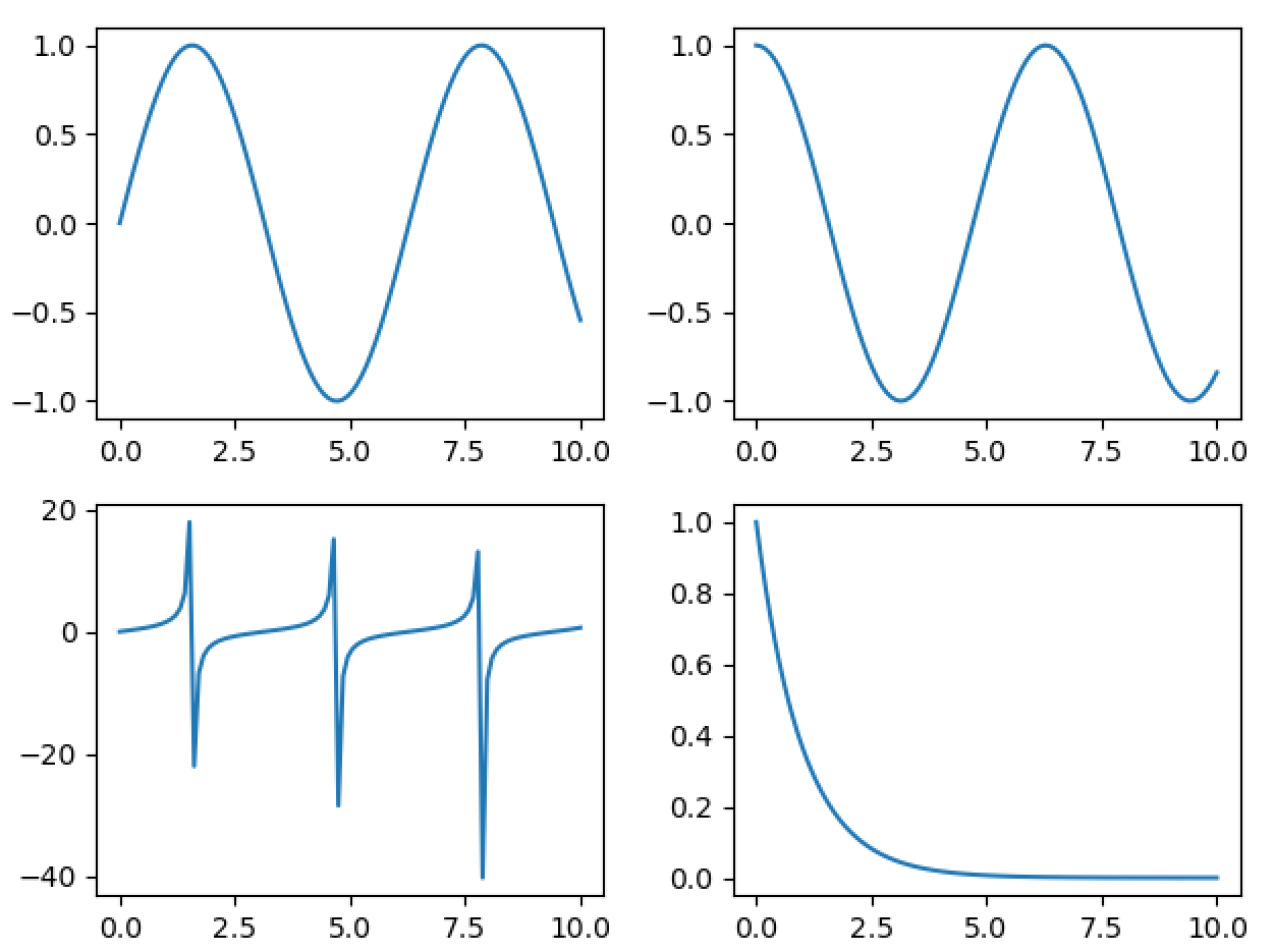
x_data = np.linspace(0, 10, 100)

# 创建四个子图
ax1 = plt.subplot(221)
ax2 = plt.subplot(222)
ax3 = plt.subplot(223)
ax4 = plt.subplot(224)

# 在每个子图中绘制不同的数据
ax1.plot(x_data, np.sin(x_data))
ax2.plot(x_data, np.cos(x_data))
ax3.plot(x_data, np.tan(x_data))
ax4.plot(x_data, np.exp(-x_data))

plt.tight_layout()
plt.show()
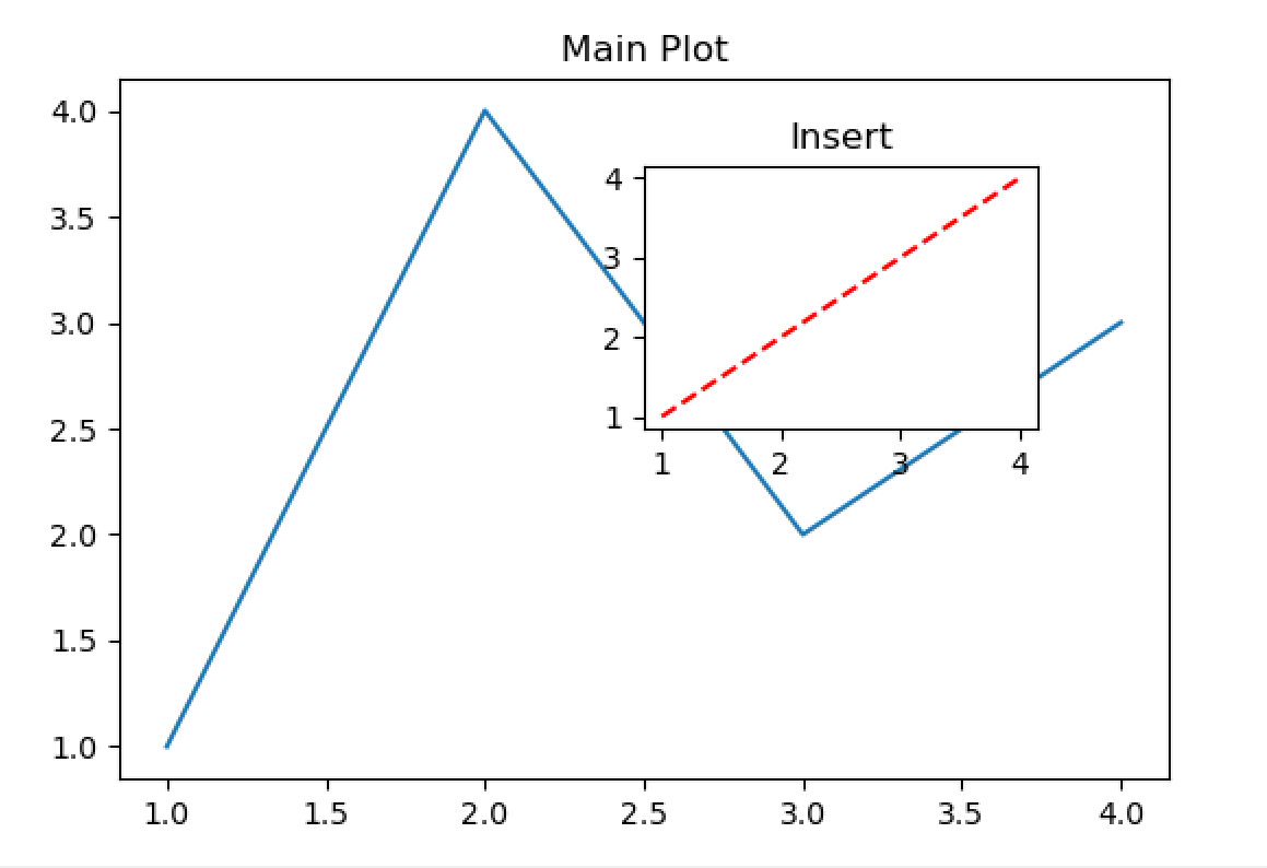
- 🍌 使用 fig.add_axes(),在指定位置添加自定义大小的 Axes,fig.add_axes(left, bottom, width, height)
– 当需要创建非常规的子图排列,例如嵌套坐标系或者大小不同的子图时,就可以使用该方法。
– 添加插入图:若要在主图内部添加一个小图来展示局部细节,就可以使用该方法。
– 精细控制位置:当你需要对子坐标系的位置进行精确控制时,就可以使用该方法。
import matplotlib.pyplot as plt

fig = plt.figure(figsize=(6, 4))

# 添加主坐标系
ax1 = fig.add_axes([0.1, 0.1, 0.8, 0.8])
ax1.plot([1, 2, 3, 4], [1, 4, 2, 3])
ax1.set_title('Main Plot')

# fig.add_axes(left, bottom, width, height)
# left:坐标系左侧边缘与图形左侧的距离比例。
# bottom:坐标系下侧边缘与图形底部的距离比例。
# width:坐标系的宽度占图形宽度的比例。
# height:坐标系的高度占图形高度的比例。
ax2 = fig.add_axes([0.5, 0.5, 0.3, 0.3])  # 位置相对于图形
ax2.plot([1, 2, 3, 4], [1, 2, 3, 4], 'r--')
ax2.set_title('Insert')

plt.show()
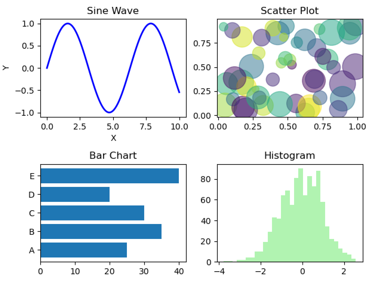
Axes基本绘图功能
-🍐 折线图(plot),折线图一般用于展示数据随连续变量(如时间)的变化趋势。
-🍐 散点图(scatter),散点图主要用于展示两个变量之间的关系,还能通过颜色或大小来表示第三个变量。
-🍐 柱状图(bar/barh),柱状图适用于比较不同类别之间的数据差异。
-🍐 直方图(hist),直方图可用于展示数据的分布情况。
import matplotlib.pyplot as plt
import numpy as np

x0 = np.linspace(0, 10, 100)
y0 = np.sin(x0)

fig, ax_old = plt.subplots(2, 2)
ax = ax_old.flatten()
ax[0].plot(x0, y0, 'b-', lw=2)  # 蓝色实线,线宽为2
ax[0].set_title('Sine Wave')
ax[0].set_xlabel('X')
ax[0].set_ylabel('Y')

x1 = np.random.rand(50)
y1 = np.random.rand(50)
colors = np.random.rand(50)
sizes = 1000 * np.random.rand(50)

ax[1].scatter(x1, y1, c=colors, s=sizes, alpha=0.5)  # alpha 为透明度
ax[1].set_title('Scatter Plot')

categories = ['A', 'B', 'C', 'D', 'E']
values = [25, 35, 30, 20, 40]

# ax[2].bar(categories, values, color='skyblue')  # 垂直柱状图
ax[2].barh(categories, values)  # 水平柱状图
ax[2].set_title('Bar Chart')

data = np.random.randn(1000)
ax[3].hist(data, bins=30, color='lightgreen', alpha=0.7)
ax[3].set_title('Histogram')
fig.tight_layout()
plt.show()
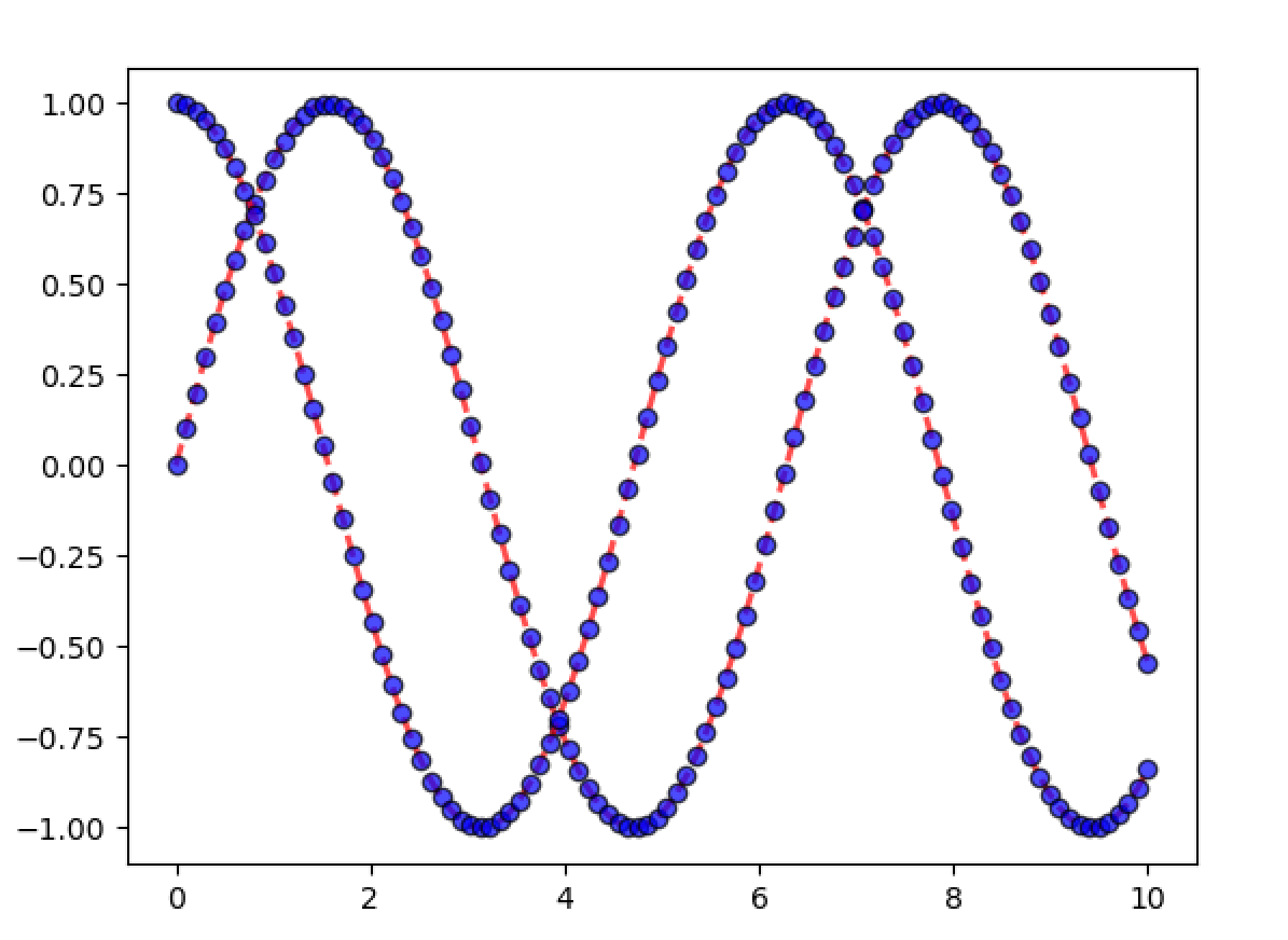
Axes绘图的常用参数
| 参数 | 说明 | 示例 |
|---|---|---|
| color,c | 颜色:支持名称、RGB、HTML 颜色代码 | color=‘red’ |
| linestyle,ls | 线型:‘-’, ‘–’, ‘-.’, ‘:’, ‘None’ | linestyle=‘–’,ls=“–” |
| linewidth, lw | 线宽 | linewidth=2 |
| marker | 标记:‘o’, ‘s’, ‘^’, ‘x’, ‘+’ | marker=‘o’ |
| markersize, ms | 标记大小 | markersize=6 |
| markerfacecolor,mfc | 标记填充色 | markerfacecolor=‘blue’ |
| markeredgecolor,mec | 标记边框色 | markeredgecolor=‘black’ |
| alpha | 透明度 | alpha=0.7 |
| label | 图例标签 | label=‘Sine’ |
import matplotlib.pyplot as plt
import numpy as np

x = np.linspace(0, 10, 100)
y0 = np.sin(x)
y1 = np.cos(x)

fig, ax = plt.subplots()
ax.plot(x, y0, x, y1,
        color='red',           # 颜色:支持名称、RGB、HTML 颜色代码, color可简写为c
        linestyle='--',        # 线型:'-', '--', '-.', ':', 'None', linestyle简写为ls
        linewidth=2,           # 线宽, linewidth简写为lw
        marker='o',            # 标记:'o', 's', '^', 'x', '+'
        markersize=6,          # 标记大小, markersize简写为ms
        markerfacecolor='blue',# 标记填充色, markerfacecolor简写为mfc
        markeredgecolor='black',# 标记边框色, markeredgecolor简写为mec
        alpha=0.7,             # 透明度
        label='Sine')           # 图例标签
plt.show()
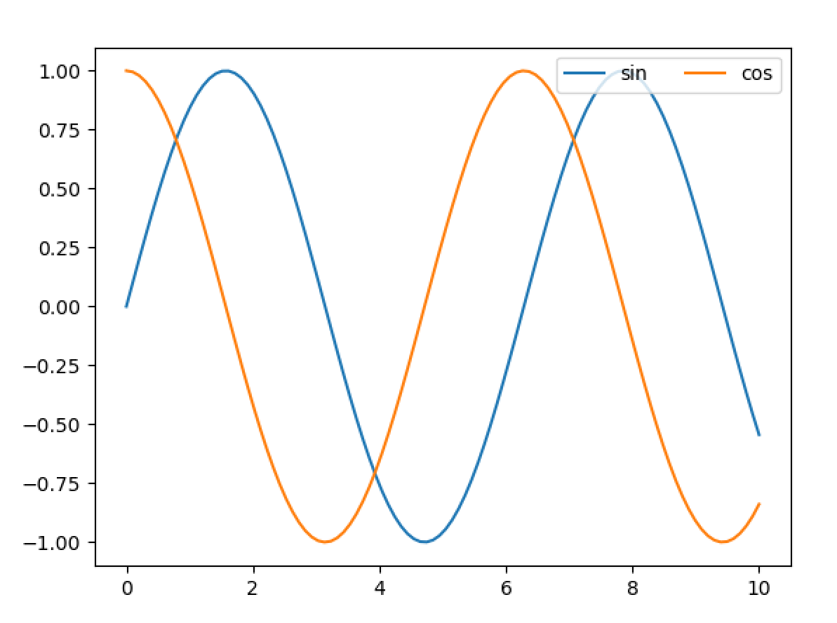
Axes图例参数
| 参数 | 说明 | 示例 |
|---|---|---|
| loc | 位置:‘best’, ‘upper right’, ‘lower left’ 等 | loc=‘lower right’ |
| frameon | 显示图例边框 | frameon=True |
| framealpha | 边框透明度 | framealpha=0.8 |
| shadow | 添加阴影 | shadow=True |
| fontsize | 字体大小 | fontsize=10 |
| ncol | 图例分栏数 | ncol=2 |
import matplotlib.pyplot as plt
import numpy as np

x = np.linspace(0, 10, 100)
y0 = np.sin(x)
y1 = np.cos(x)

fig, ax = plt.subplots()
ax.plot(x, y0, label="sin")
ax.plot(x, y1, label="cos")
ax.legend(
    loc='upper right',    # 位置:'best', 'upper right', 'lower left' 等
    frameon=True,         # 显示图例边框
    framealpha=0.8,       # 边框透明度
    shadow=False,         # 添加阴影
    fontsize=10,          # 字体大小
    ncol=2)               # 图例分栏数
plt.show()
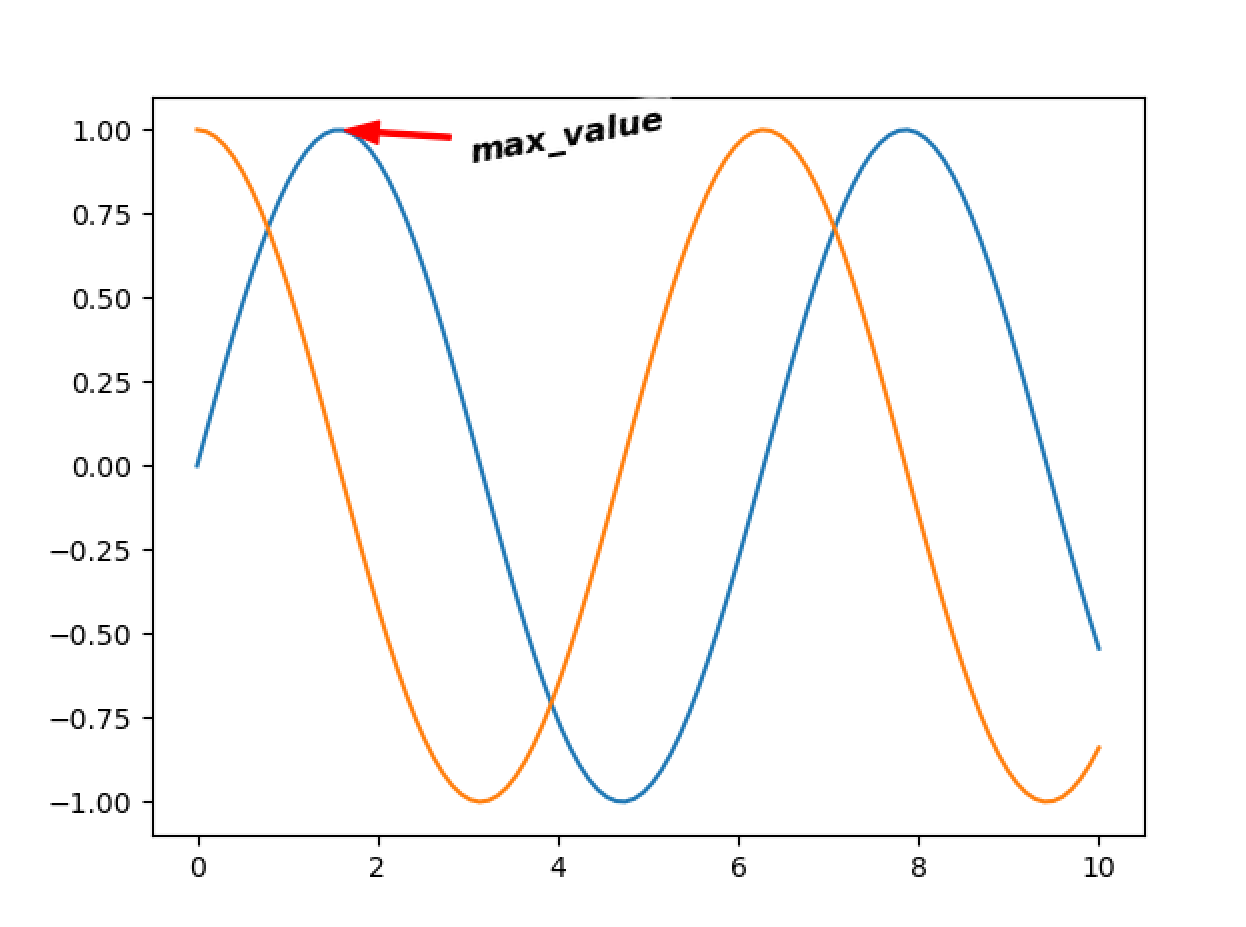
Axes注释参数
- 🍉 annotate(text, xy, xytext=None, xycoords=‘data’, textcoords=None,
arrowprops=None, bbox=None, **kwargs)
| 参数 | 说明 | 示例 |
|---|---|---|
| text | 注释文本内容 | ‘最大值’, f’温度: {temp}°C’ |
| xy | 箭头指向的点坐标(x, y) | (2.5, 3.7) |
| xytext | 文本的位置坐标(默认与 xy 相同) | (4, 3) 或 (30, -20)(若使用偏移量) |
| xycoords | xy 的坐标系类型 | ‘data’(默认,数据坐标)‘axes fraction’(轴比例) |
| textcoords | xytext 的坐标系类型(若为偏移量,需设置为 ‘offset points’) | ‘offset points’(像素偏移)、‘data’ |
注释箭头参数(arrowprops)
- 🍉 通过字典传递, arrowprops=dict()
| 参数 | 说明 | 示例 |
|---|---|---|
| arrowstyle | 箭头样式 ‘-’(无箭头)、‘->’(单线箭头)、‘simple’(实心箭头) | |
| color | 箭头颜色 | color =‘black’, ‘#FF0000’ |
| edgecolor | 箭头框颜色 | edgecolor=‘red’ |
| width | 箭身宽度(点为单位)width = 1.5 | |
| headwidth | 箭头宽度(点为单位) | headwidth =8 |
| shrink | 箭头两端与 xy 和 xytext 的距离(比例值) | 0.05(表示收缩 5%) |
| connectionstyle | 连接样式(用于弯曲箭头) | ‘arc3,rad=0.3’(弧度为 0.3 的曲线) |
文本框参数(bbox)
- 🍉 控制文本周围的边框样式,通过字典传递, bbox=dict()
| 参数 | 说明 | 示例 |
|---|---|---|
| boxstyle | 边框样式 ‘round’(圆角) | ‘square,pad=0.5’(方角,内边距 0.5) |
| facecolor | 背景颜色 | ‘white’, ‘yellow’, (1,1,1,0.5)(带透明度) |
| edgecolor | 边框颜色 | ‘black’, ‘red’ |
| alpha | 透明度 | 0.5 |
其它注释参数
| 参数 | 说明 | 示例 |
|---|---|---|
| fontsize | 文本字体大小 | 12, ‘large’ |
| fontweight | 文本字体粗细 | ‘bold’, ‘normal’ |
| color | 文本颜色 | ‘blue’, ‘#00FF00’ |
| ha / horizontalalignment | 文本水平对齐方式 | ‘center’, ‘left’, ‘right’ |
| va / verticalalignment | 文本垂直对齐方式 | ‘center’, ‘bottom’, ‘top’ |
| rotation | 文本旋转角度(度) | 45, ‘vertical’ |
x = np.linspace(0, 10, 100)
y0 = np.sin(x)
y1 = np.cos(x)
plt.plot(x, y0, x, y1)

plt.annotate('max_value',
            xy=(1.57, 1),  # 注释点坐标
            xytext=(3, 0.8),  # 文本位置
            arrowprops=dict(
                color='red',  # 箭头颜色
                edgecolor='red',  # 箭头框颜色
                shrink=0.05,  # 箭头与文本的距离
                width=1.5,  # 箭身宽度
                headwidth=8  # 箭头宽度
            ),
            fontsize=12, fontweight="bold", fontstyle='italic', rotation=10,
            bbox=dict(boxstyle="round,pad=0.3", fc="white", ec="white", alpha=0.5)
            )
plt.show()
Axes的常用方法
基本设置
| 方法 | 说明 | 示例 |
|---|---|---|
| title | 设置子图标题 | ax.set_title(‘Temperature Plot’) |
| xlabel, ylabel | 设置坐标轴标签 | ax.set_xlabel(‘Time (s)’) |
| xlim, ylim | 设置坐标轴范围 | ax.set_xlim(0, 10) |
| xticks, yticks | 设置刻度位置和标签 | ax.set_xticks([0, 5, 10]) |
| set_xticklabels | 设置刻度标签 | ax.set_xticklabels([‘a’, ‘b’, ‘c’, ‘d’, ‘e’, ‘f’]) |
| flatten | 将axes如果是2维的,变成1维进行访问,ax[1,1]变成ax[3],便于书写和循环 | axes.flattern() |
刻度与网格边框
| 方法 | 说明 | 示例 |
|---|---|---|
| tick_params | 自定义刻度样式 | ax.tick_params(axis=‘x’, rotation=45) |
| grid | 显示 / 隐藏网格线 | ax.grid(True, linestyle=‘–’) |
| spines | 控制坐标轴边框 | ax.spines[‘top’].set_visible(False) |
图例与注释
| 方法 | 说明 | 示例 |
|---|---|---|
| legend | 添加图例 | ax.legend([‘Data 1’, ‘Data 2’]) |
| text | 在指定位置添加文本 | ax.text(2, 5, ‘Peak Value’) |
| annotate | 添加带箭头的注释 | ax.annotate(‘Max’, xy=(3, 10), arrowprops=dict(facecolor=‘black’)) |
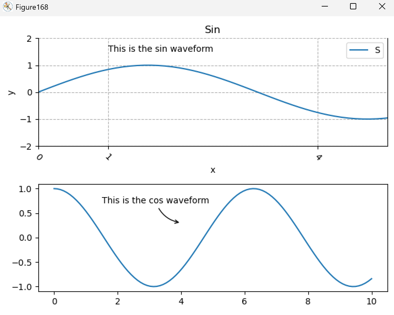
code:
import matplotlib.pyplot as plt
import numpy as np

fig, ax = plt.subplots(2, 1, num="Figure168")
x = np.linspace(0, 10, 100)
y1 = np.sin(x)
y2 = np.cos(x)
ax[0].plot(x, y1)
ax[1].plot(x, y2)

ax[0].spines["top"].set_visible(False)
ax[0].tick_params(axis='x', rotation=315)
ax[0].set_xticks([0, 1, 4])
ax[0].set_title("Sin")
ax[0].set_xlabel("x")
ax[0].set_ylabel("y")
ax[0].set_xlim(0, 5)
ax[0].set_ylim(-2, 2)
ax[0].legend("Sine Waveform")
ax[0].grid(True, linestyle='--')
ax[0].text(1, 1.5, 'This is the sin waveform')
ax[1].annotate('This is the cos waveform', xy=(4, 0.3), xytext=(1.5,0.7),
            arrowprops=dict(arrowstyle='->',
                            connectionstyle='arc3,rad=0.3'))
plt.tight_layout()
print(ax[0].get_title(), ax[0].get_xlabel(), ax[0].get_ylabel(), ax[0].get_xlim(), ax[0].get_ylim())

result:
Sin x y (0.0, 5.0) (-2.0, 2.0)
图形样式
| 方法 | 说明 | 示例 |
|---|---|---|
| facecolor | 设置绘图区背景颜色 | ax.set_facecolor(‘#f0f0f0’) |
| alpha | 设置透明度 | ax.set_alpha(0.8) |
| aspect | 设置坐标轴纵横比 | ax.set_aspect(‘equal’) |
| twinx, twiny | 创建共享坐标轴的双 Y 轴 / 双 X 轴 | ax2 = ax.twinx() |
Axis(坐标轴)
- 🍎 Axes 的一部分,控制单个坐标轴的具体属性(如刻度、标签、范围)。
- 🍎 设置刻度位置(ticks)和标签(ticklabels)。
- 🍎 控制坐标轴范围(如xlim、ylim)。
- 🍎 管理坐标轴的缩放类型(线性、对数等)。
获取axis对象
- 🍓 ax.xaxis, ax.yaxis
刻度位置(Locator)
- 🍓 MultipleLocator(base):固定间隔刻度(如 base=0.5 表示每 0.5 一个刻度)
- 🍓 MaxNLocator(nbins):自动选择最多 nbins 个刻度
- 🍓 FixedLocator(locs):自定义刻度位置(如 [1, 3, 5])
- 🍓 AutoLocator():自动定位(默认选项)
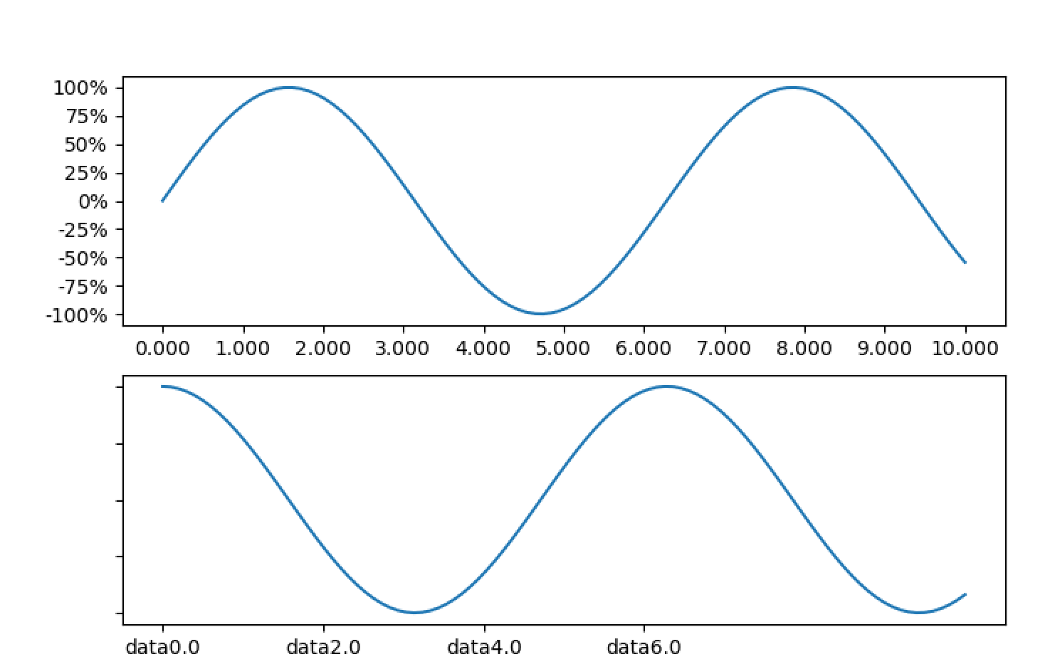
刻度格式(Formatter)
- 🍓 PercentFormatter(xmax):百分比格式(如 xmax=1.0 时,0.5 → 50%)
- 🍓 StrMethodFormatter(“{x:.2f}”):自定义字符串格式
- 🍓 FuncFormatter(func):自定义函数格式化
- 🍓 NullFormatter():不显示刻度标签
code:
import matplotlib.pyplot as plt
import numpy as np
from matplotlib.ticker import PercentFormatter, StrMethodFormatter, FuncFormatter, NullFormatter
from matplotlib.ticker import MultipleLocator, MaxNLocator, FixedLocator, AutoLocator

fig, ax = plt.subplots(2, 1, figsize=(8, 5))

# 获取x轴和y轴
x0_axis = ax[0].xaxis
y0_axis = ax[0].yaxis
x1_axis = ax[1].xaxis
y1_axis = ax[1].yaxis

# 设置刻度位置
x0_axis.set_major_locator(MultipleLocator(1))  # 每1一个刻度
y0_axis.set_major_locator(MaxNLocator(10))  # 一共10个刻度值
x1_axis.set_major_locator(FixedLocator([0, 2, 4, 6]))  # 固定的数值作为locator
y1_axis.set_major_locator(AutoLocator())  # 自动设置

def data_covert(x, pos):  # pos: 刻度位置
    return f'data{x:.1f}'

# 设置刻度格式
x0_axis.set_major_formatter(StrMethodFormatter("{x:.3f}"))  # 自定义字符串格式
y0_axis.set_major_formatter(PercentFormatter(xmax=1.0))  # 百分比格式

x1_axis.set_major_formatter(FuncFormatter(data_covert))  # FuncFormatter(func):自定义函数格式化
y1_axis.set_major_formatter(NullFormatter())  # NullFormatter():不显示刻度标签

x = np.linspace(0,10, 100)
y0 = np.sin(x)
y1 = np.cos(x)
ax[0].plot(x, y0)
ax[1].plot(x, y1)

plt.show()
隐藏坐标轴或刻度
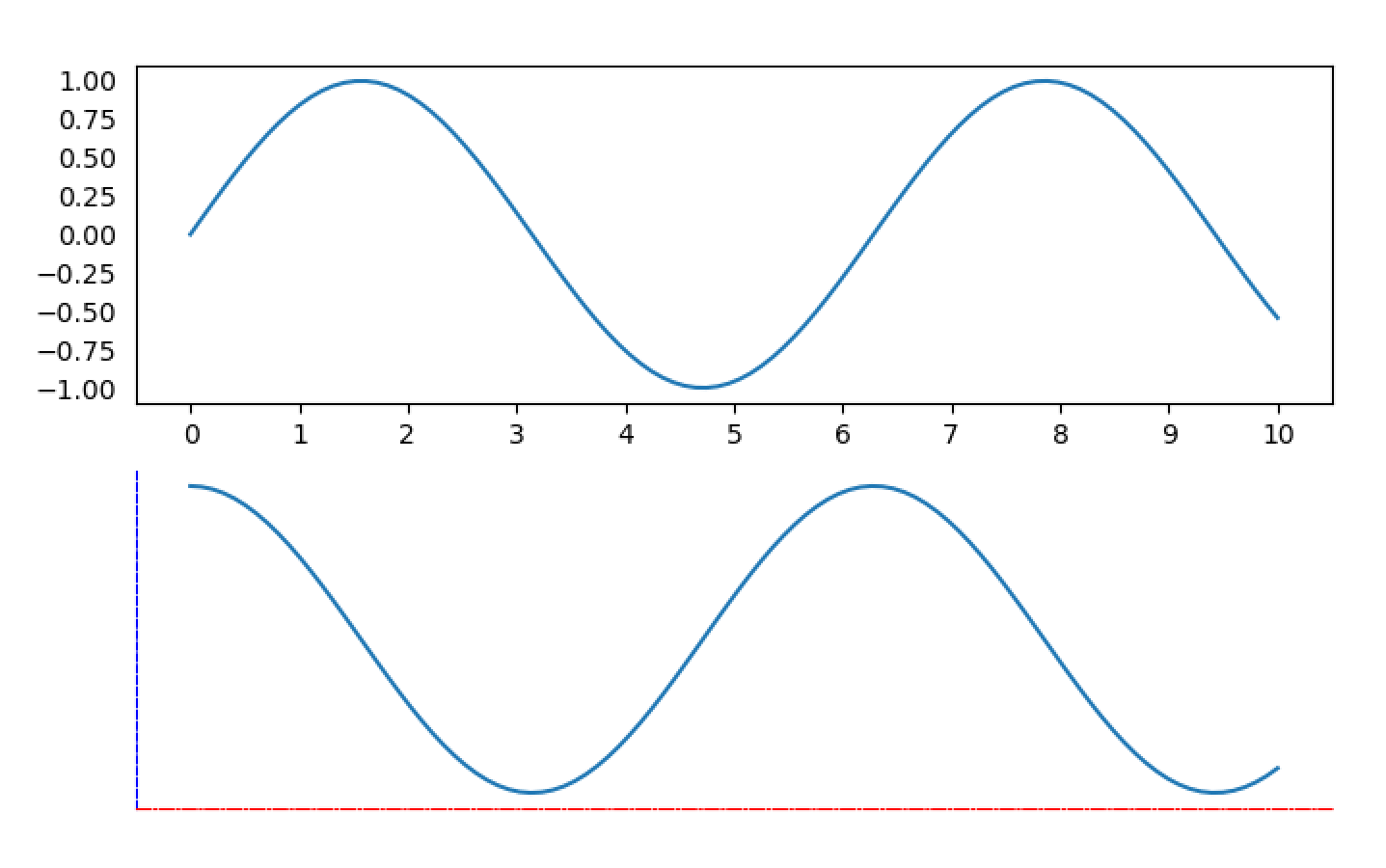
隐藏刻度
- 🍉 隐藏y轴的刻度,使用tick_params
– x1_axis.set_visible(False) # 隐藏刻度
– y1_axis.set_visible(False) # 隐藏刻度 - 🍉 隐藏y轴的刻度,使用tick_params
– ax[0].tick_params(axis=‘x’, which=‘both’, bottom=True, labelbottom=True) # ‘minor’, ‘major’, ‘both’
– ax[0].tick_params(axis=‘y’, which=‘both’, left=False, labelbottom=True)
隐藏边框和设置边框
- 🥒 ax[1].spines[‘top’].set_visible(False) # 隐藏边框
- 🥒 ax[1].spines[‘right’].set_visible(False) # 隐藏边框
- 🥒 ax[0].set_frame_on(False) # 隐藏所有边框
- 🥒 设置边框
– ax[1].spines[‘left’].set_linestyle(‘–’) # 设置边框线型
– ax[1].spines[‘bottom’].set_linestyle(‘-.’)
– ax[1].spines[‘left’].set_color(‘blue’) # 设置边框颜色
– ax[1].spines[‘bottom’].set_color(‘red’)
code:
import matplotlib.pyplot as plt
import numpy as np
from matplotlib.ticker import MultipleLocator, MaxNLocator

fig, ax = plt.subplots(2, 1, figsize=(8, 5))

# 获取x轴和y轴
x0_axis = ax[0].xaxis
y0_axis = ax[0].yaxis
x1_axis = ax[1].xaxis
y1_axis = ax[1].yaxis

# 设置刻度位置
x0_axis.set_major_locator(MultipleLocator(1))  # 每1一个刻度
y0_axis.set_major_locator(MaxNLocator(10))  # 一共10个刻度值

x1_axis.set_visible(False)  # 隐藏刻度
y1_axis.set_visible(False)  # 隐藏刻度

# 隐藏y轴的刻度,使用tick_params
ax[0].tick_params(axis='x', which='both', bottom=True, labelbottom=True) # 'minor', 'major', 'both'
ax[0].tick_params(axis='y', which='both', left=False, labelbottom=True)

# 隐藏边框
ax[1].spines['top'].set_visible(False)  # 隐藏边框
ax[1].spines['right'].set_visible(False)  # 隐藏边框
# ax[0].set_frame_on(False)  # 隐藏所有边框
ax[1].spines['left'].set_linestyle('--')  # 设置边框线型
ax[1].spines['bottom'].set_linestyle('-.')
ax[1].spines['left'].set_color('blue')  # 设置边框颜色
ax[1].spines['bottom'].set_color('red')

x = np.linspace(0,10, 100)
y0 = np.sin(x)
y1 = np.cos(x)
ax[0].plot(x, y0)
ax[1].plot(x, y1)
plt.show()
自定义刻度外观
- 🍍 ax.tick_params设置
code:
ax.tick_params(
    axis='both',         # 同时设置 X 和 Y 轴
    which='major',       # 只设置主刻度
    length=5,            # 刻度线长度
    width=1,             # 刻度线宽度
    labelsize=10,        # 标签字体大小
    direction='in',      # 刻度线方向(in、out、inout)
    color='red',         # 刻度线颜色
    labelcolor='blue'    # 标签颜色
)
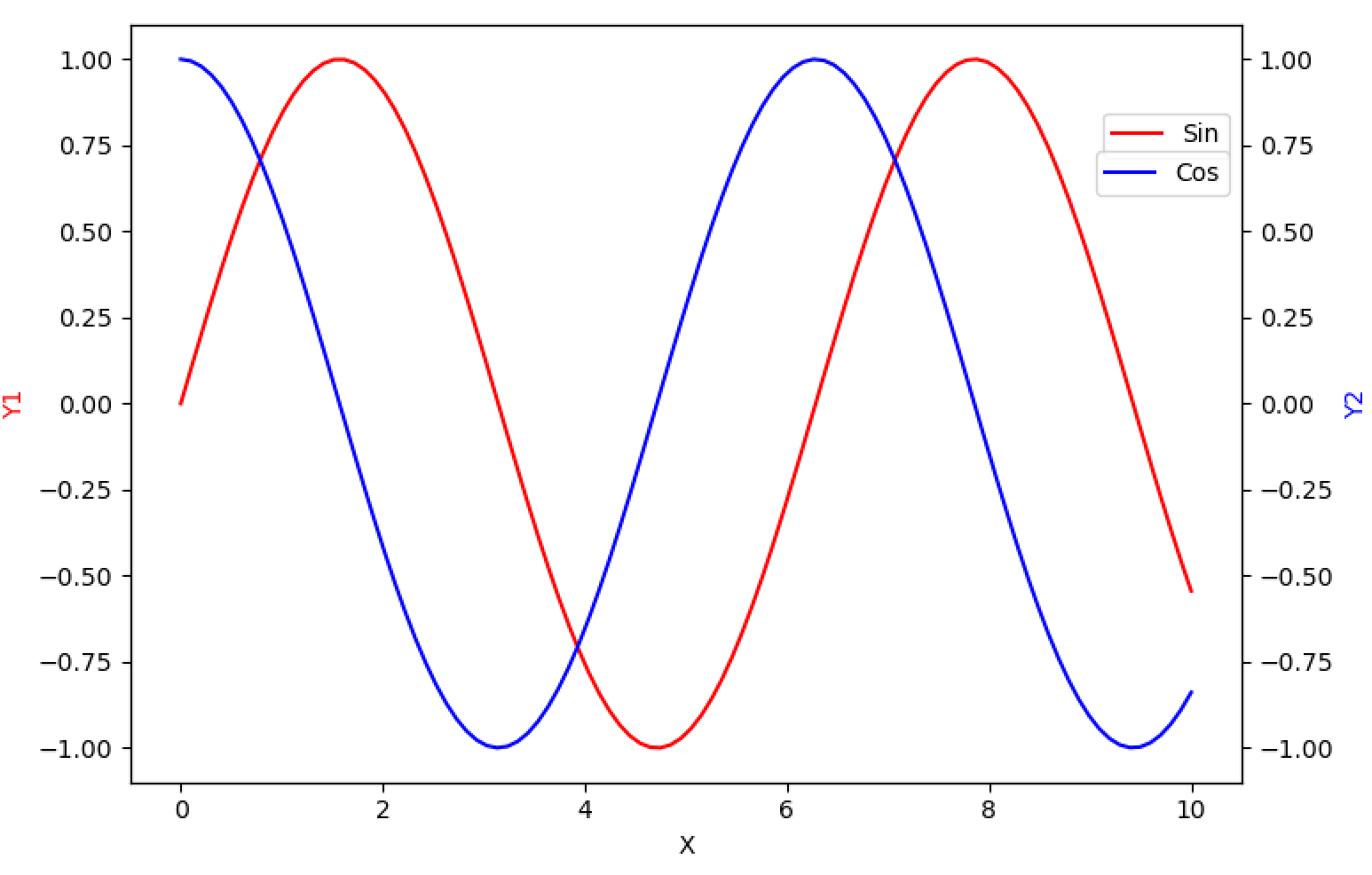
共享X轴
-🌹 类似于在excel中将另一个图画在次坐标轴, 设置一个ax1对象,第二个ax直接ax2 = ax1.twinx()
-🌹 正常的只建立一个ax,第二个ax直接ax2 = ax1.twinx(),然后画图
code:
import matplotlib.pyplot as plt
import numpy as np

# 类似于在excel中将另一个图画在次坐标轴, 设置一个ax1对象,第二个ax直接ax2 = ax1.twinx()
fig, ax1 = plt.subplots(figsize=(8, 5))
x = np.linspace(0, 10, 100)
y1 = np.sin(x)
y2 = np.cos(x)

# 第一个 Y 轴
ax1.set_xlabel('X')
ax1.set_ylabel('Y1', color='red')
ax1.plot(x, y1, color='red')

# 第二个 Y 轴(共享 X 轴)
ax2 = ax1.twinx()
ax2.set_ylabel('Y2', color='blue')
ax2.plot(x, y2, color='blue')

plt.show()
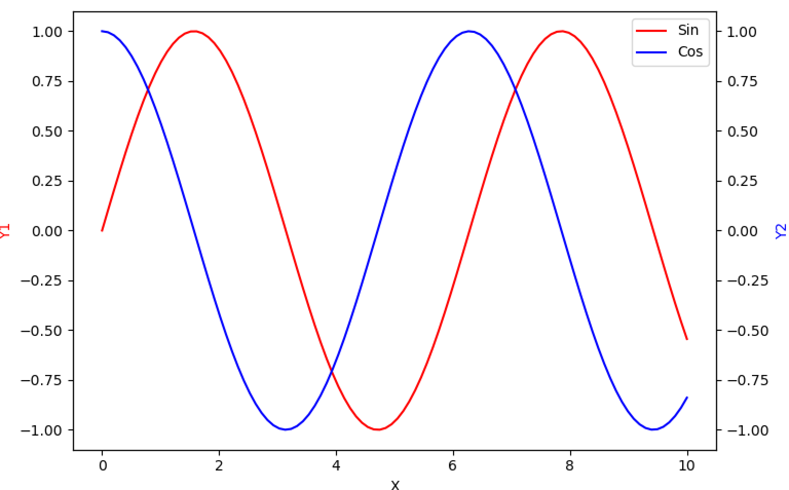
共享X轴时的legend设置
-🌹 设置图例时,由于分别属于不同的ax,单独显示在同一位置时会覆盖。
-🌹 可以将两个图的线条和图例合并在一起,在某一个ax上显示。
-🌹 虽然是数轴的内容,但是通过axes设置。
code:
import matplotlib.pyplot as plt
import numpy as np

# 类似于在excel中将另一个图画在次坐标轴, 设置一个ax1对象,第二个ax直接ax2 = ax1.twinx()
fig, ax1 = plt.subplots(figsize=(8, 5))
x = np.linspace(0, 10, 100)
y1 = np.sin(x)
y2 = np.cos(x)

# 第一个 Y 轴
ax1.set_xlabel('X')
ax1.set_ylabel('Y1', color='red')
ax1.plot(x, y1, color='red', label='Sin')
# ax1.legend(loc='lower right')  # 显示第一个图例,单独显示
# 第二个 Y 轴(共享 X 轴)
ax2 = ax1.twinx()
ax2.set_ylabel('Y2', color='blue')
ax2.plot(x, y2, color='blue', label='Cos')
# ax2.legend(loc='upper left')  # 显示第二个图例,单独显示

# 同时显示两个图例, 都在某一个ax上显示,另一个的ax不显示
# 将两个子图的线条和标签收集起来,创建一个统一的图例:
lines1, labels1 = ax1.get_legend_handles_labels()
lines2, labels2 = ax2.get_legend_handles_labels()
ax2.legend(lines1 + lines2, labels1 + labels2, loc='upper right')

plt.tight_layout()
plt.show()
import matplotlib.pyplot as plt
import numpy as np

# 类似于在excel中将另一个图画在次坐标轴, 设置一个ax1对象,第二个ax直接ax2 = ax1.twinx()
fig, ax1 = plt.subplots(figsize=(8, 5))
x = np.linspace(0, 10, 100)
y1 = np.sin(x)
y2 = np.cos(x)

ax1.set_xlabel('X')
ax1.set_ylabel('Y1', color='red')
ax1.plot(x, y1, color='red', label='Sin')

ax2 = ax1.twinx()
ax2.set_ylabel('Y2', color='blue')
ax2.plot(x, y2, color='blue', label='Cos')

# 分别放置图例
ax1.legend(loc='upper right', bbox_to_anchor=(1, 0.9))  # 上方
ax2.legend(loc='upper right', bbox_to_anchor=(1, 0.85))  # 上方

plt.tight_layout()
plt.show()
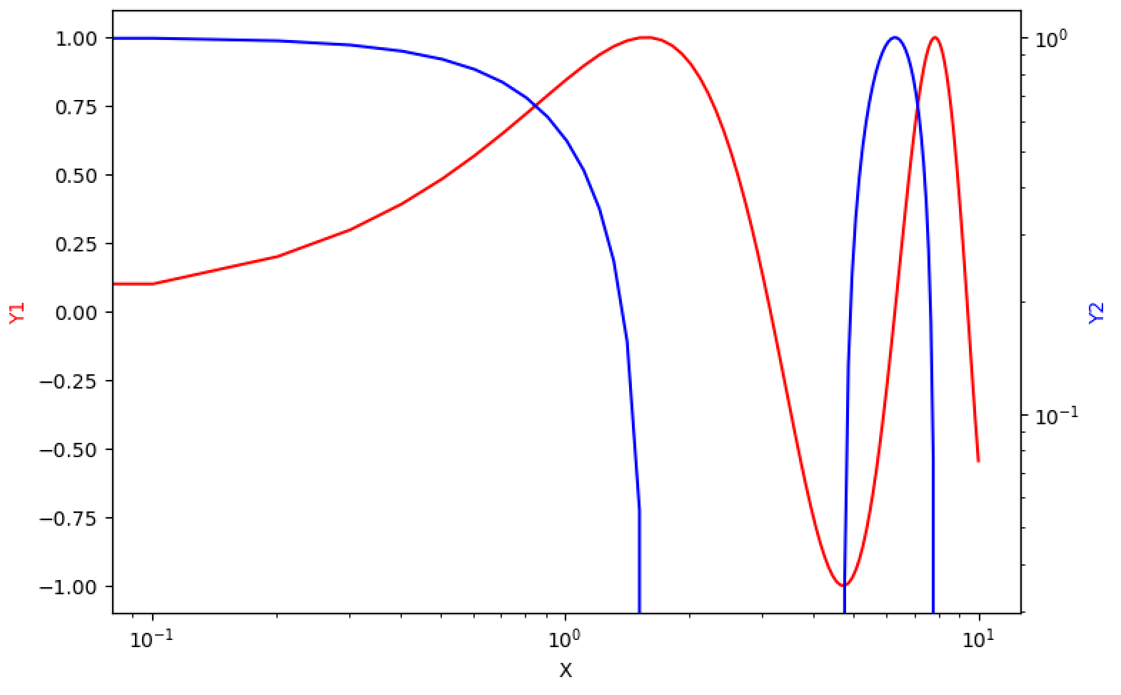
设置对数坐标
- 🍓 虽然是数轴的东西,但是通过axes设置。
- 🍓 ax2.set_yscale(‘log’)色设置对数坐标。
mport matplotlib.pyplot as plt
import numpy as np
# 类似于在excel中将另一个图画在次坐标轴, 设置一个ax1对象,第二个ax直接ax2 = ax1.twinx()
fig, ax1 = plt.subplots(figsize=(8, 5))
x = np.linspace(0, 10, 100)
ax1.set_xscale('log')  # X 轴为对数刻度

y1 = np.sin(x)
y2 = np.cos(x)

ax1.set_xlabel('X')
ax1.set_ylabel('Y1', color='red')
ax1.plot(x, y1, color='red', label='Sin')

ax2 = ax1.twinx()
ax2.set_ylabel('Y2', color='blue')
ax2.set_yscale('log')  # X 轴为对数刻度
ax2.plot(x, y2, color='blue', label='Cos')

plt.tight_layout()
plt.show()
axes和axis的对比
- 🌼 有些关于axis的性质要通过axes的方法取设置。
| 方法 | 说明 | 示例 |
|---|---|---|
| 维度 | Axes | Axis |
| 层级关系 | 属于 Figure,包含两个或三个 Axis 对象 | 属于 Axes,是其组成部分,但是多个axes可以共享一个axis |
| 实例数量 | 一个 Figure 可包含多个 Axes(如 2×2 网格有 4 个 Axes) | 每个 Axes 至少包含 X 轴和 Y 轴或 X、Y、Z 轴 |
| 绘图操作 | 通过plot()、scatter()等方法绘制数据 | 无直接绘图方法,主要控制坐标轴属性 |
| 属性设置 | 设置标题、图例、网格等全局元素 | 设置刻度、标签、范围等坐标轴特定元素 |
| 访问方式 | fig, axes = plt.subplots(2, 2)返回 Axes 数组 | ax.xaxis或ax.yaxis访问特定 Axis 对象 |

![[ Qt ] | QPushButton常见用法](https://i-blog.csdnimg.cn/direct/334f8a5a97c54445aae4804912a67fcf.png)