【 声明：版权所有，欢迎转载，请勿用于商业用途。 联系信箱：feixiaoxing @163.com】

        对于slam而言，大家一般想到的就是去通过传感器找特征点，进而借助于特征点去定位机器人的位置。但是对于用户或者厂家来说，他们很多时候对机器人在道路上的精度不做要求，但对工位上的对接要求很高。所以，对于供应商来说，是不是整个定位和导航都需要借助于传感器或者反光柱，这就两说了。

        此外，相比较室外而言，工厂内部的光源一般会好一点。就算条件不是很好，我们自己也可以通过补充光源的形式加以修正。所以，对于机器人来说，一种不错的导航方法就是借助于路面来机器人的自我定位，相信也是可以考虑的一个选择。

        网上关于车道线检测的代码不少，我们不妨找一个来学习和参考下，之前文章的地址如下，

https://www.cnblogs.com/wojianxin/p/12624096.html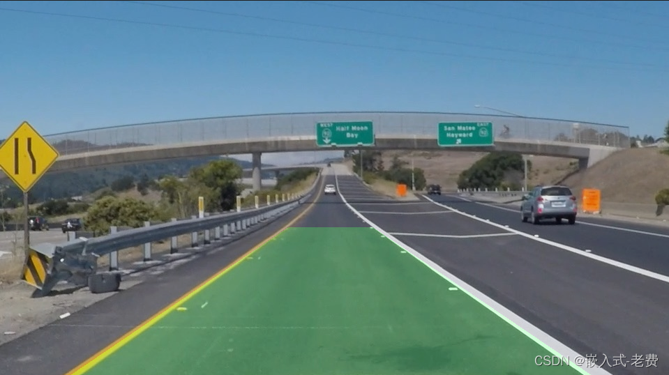

1、图像灰化，提取边缘信息

    # 1. 灰度化、滤波和Canny
    gray = cv.cvtColor(img, cv.COLOR_RGB2GRAY)
    blur_gray = cv.GaussianBlur(gray, (blur_ksize, blur_ksize), 1)
    edges = cv.Canny(blur_gray, canny_lth, canny_hth)

2、兴趣区域截取

    # 2. 标记四个坐标点用于ROI截取
    rows, cols = edges.shape
    points = np.array([[(0, rows), (460, 325), (520, 325), (cols, rows)]])
    # [[[0 540], [460 325], [520 325], [960 540]]]
    roi_edges = roi_mask(edges, points)

3、利用HoughLinesP函数提取直线

    # 3. 霍夫直线提取
    drawing, lines = hough_lines(roi_edges, rho, theta,
                                 threshold, min_line_len, max_line_gap)

4、车道线拟合

        生成的车道线很多，这个步骤主要是将多个车道线拟合成左右各两条直线。其中左边直线的斜率大于等于0，右边直线的斜率小于等于0。整个拟合的过程中使用到了最小二乘法。

    # 4. 车道拟合计算
    draw_lanes(drawing, lines)

5、绘制车道线

        拟合出来的车道线，最终需要放到原来的图片上，验证一下实现的效果。

    # 5. 最终将结果合在原图上
    result = cv.addWeighted(img, 0.9, drawing, 0.2, 0)

6、完整的代码

import cv2 as cv
import numpy as np

# 高斯滤波核大小
blur_ksize = 5

# Canny边缘检测高低阈值
canny_lth = 50
canny_hth = 150

# 霍夫变换参数
rho = 1
theta = np.pi / 180
threshold = 15
min_line_len = 40
max_line_gap = 20


def process_an_image(img):
    # 1. 灰度化、滤波和Canny
    gray = cv.cvtColor(img, cv.COLOR_RGB2GRAY)
    blur_gray = cv.GaussianBlur(gray, (blur_ksize, blur_ksize), 1)
    edges = cv.Canny(blur_gray, canny_lth, canny_hth)

    # 2. 标记四个坐标点用于ROI截取
    rows, cols = edges.shape
    points = np.array([[(0, rows), (460, 325), (520, 325), (cols, rows)]])
    # [[[0 540], [460 325], [520 325], [960 540]]]
    roi_edges = roi_mask(edges, points)

    # 3. 霍夫直线提取
    drawing, lines = hough_lines(roi_edges, rho, theta,
                                 threshold, min_line_len, max_line_gap)

    # 4. 车道拟合计算
    draw_lanes(drawing, lines)

    # 5. 最终将结果合在原图上
    result = cv.addWeighted(img, 0.9, drawing, 0.2, 0)

    return result


def roi_mask(img, corner_points):
    # 创建掩膜
    mask = np.zeros_like(img)
    cv.fillPoly(mask, corner_points, 255)

    masked_img = cv.bitwise_and(img, mask)
    return masked_img


def hough_lines(img, rho, theta, threshold, min_line_len, max_line_gap):
    # 统计概率霍夫直线变换
    lines = cv.HoughLinesP(img, rho, theta, threshold,
                            minLineLength=min_line_len, maxLineGap=max_line_gap)

    # 新建一副空白画布
    drawing = np.zeros((img.shape[0], img.shape[1], 3), dtype=np.uint8)
    # 画出直线检测结果
    # draw_lines(drawing, lines)
    # print(len(lines))

    return drawing, lines


def draw_lines(img, lines, color=[0, 0, 255], thickness=1):
    for line in lines:
        for x1, y1, x2, y2 in line:
            cv.line(img, (x1, y1), (x2, y2), color, thickness)


def draw_lanes(img, lines, color=[255, 0, 0], thickness=8):
    # a. 划分左右车道
    left_lines, right_lines = [], []
    for line in lines:
        for x1, y1, x2, y2 in line:
            k = (y2 - y1) / (x2 - x1)
            if k < 0:
                left_lines.append(line)
            else:
                right_lines.append(line)

    if (len(left_lines) <= 0 or len(right_lines) <= 0):
        return

    # b. 清理异常数据
    clean_lines(left_lines, 0.1)
    clean_lines(right_lines, 0.1)

    # c. 得到左右车道线点的集合，拟合直线
    left_points = [(x1, y1) for line in left_lines for x1, y1, x2, y2 in line]
    left_points = left_points + [(x2, y2)
                                 for line in left_lines for x1, y1, x2, y2 in line]

    right_points = [(x1, y1)
                    for line in right_lines for x1, y1, x2, y2 in line]
    right_points = right_points + \
        [(x2, y2) for line in right_lines for x1, y1, x2, y2 in line]

    left_results = least_squares_fit(left_points, 325, img.shape[0])
    right_results = least_squares_fit(right_points, 325, img.shape[0])

    # 注意这里点的顺序
    vtxs = np.array(
        [[left_results[1], left_results[0], right_results[0], right_results[1]]])
    # d.填充车道区域
    cv.fillPoly(img, vtxs, (0, 255, 0))

    # 或者只画车道线
    # cv.line(img, left_results[0], left_results[1], (0, 255, 0), thickness)
    # cv.line(img, right_results[0], right_results[1], (0, 255, 0), thickness)


def clean_lines(lines, threshold):
    # 迭代计算斜率均值，排除掉与差值差异较大的数据
    slope = [(y2 - y1) / (x2 - x1)
             for line in lines for x1, y1, x2, y2 in line]
    while len(lines) > 0:
        mean = np.mean(slope)
        diff = [abs(s - mean) for s in slope]
        idx = np.argmax(diff)
        if diff[idx] > threshold:
            slope.pop(idx)
            lines.pop(idx)
        else:
            break


def least_squares_fit(point_list, ymin, ymax):
    # 最小二乘法拟合
    x = [p[0] for p in point_list]
    y = [p[1] for p in point_list]

    # polyfit第三个参数为拟合多项式的阶数，所以1代表线性
    fit = np.polyfit(y, x, 1)
    fit_fn = np.poly1d(fit)  # 获取拟合的结果

    xmin = int(fit_fn(ymin))
    xmax = int(fit_fn(ymax))

    return [(xmin, ymin), (xmax, ymax)]


if __name__ == "__main__":
    img = cv.imread('img02.jpg')
    result = process_an_image(img)
    cv.imshow("lane", np.hstack((img, result)))
    cv.waitKey(0)

        执行方法也非常简单，直接输入python3 checkplane.py即可。注意，这里测试的图片是img02.jpg，大家可以换成自己的测试图片。最后，非常感谢原作者给出的参考代码。