目录
前言
一、pandas常用数据类型
综述
1.一维数组(Series)与常用操作
(1) 通过列表创建Series
(2)创建Series时指定索引
(3)Series位置和标签的使用
(4)通过字典创建Series
(5)键值和指定的索引不匹配
(6)不同索引数据的自动对齐
(7)Series索引的修改
2.时间序列与常用操作
(1)创建时间序列
(2)使用日期时间做索引,创建Series对象
(3)period_range生成时间序列
3.二维表格(DataFrame)与常用操作
(1)DataFrame的创建
(2)DataFrame创建时指定列名和索引
(3)DataFrame创建时的空缺值
(4)DataFrame的属性查询
4.索引对象
(1)显示DataFrame的索引和列
(2)对DataFrame的索引和列的测试
二、pandas索引操作
1.重新索引(Series)
2.重新索引时填充缺失值(Series中)
3.缺失值的前后向填充(Series)
4.重新索引(DateFrame中)
5.重新索引, 传入fill_value=n填充缺失值(DateFrame中)
6.reindex函数参数
7.更换索引set_index函数
三、DataFrame的数据查询与编辑
1.DataFrame的数据查询
(1)选取列
(2)选取行
(3)head,tail,sample方法选取行
(4)选取行和列
(5)布尔选择
2.DataFrame的数据的编辑
(1)增加数据
(2)删除数据
(3)修改数据
四、pandas数据运算
1.算数运算
(1)series相加
(2)DataFrame类型的数据相加
2.函数应用和映射
(1)将水果价格表中的“元”去掉
(2)apply函数与applymap函数的使用方法
3.排序
(1)Series的排序
(2)DataFrame的排序
4.汇总与统计
(1)数据汇总
(2)描述与统计分析
前言
- 熟练掌握pandas一维数组series结构的使用
- 熟练掌握pandas时间序列对象的使用
- 熟练掌握pandas二维数组DataFrame结构的创建
- 熟练掌握DataFrame结构中数据的选择与查看
- 熟练掌握查看DataFrame结构中数据特征的方法
- 数量掌握DataFrame结构的排序方法
- 数量掌握DataFrame结构中数据的分组和聚合方法
- 数量掌握DataFrame结构中异常值的查看与处理
- 数量掌握DataFrame结构中缺失值的查看与处理
- 数量掌握DataFrame结构重复值的查看与处理
- 数量掌握DataFrame结构中数据差分的使用
- 熟练掌握pandas提供的透视表与交叉表技术
- 数量掌握DataFrame结构中数据的重采样技术
一、pandas常用数据类型
综述
扩展库pandas是基于扩展库numpy和matplotlib的数据分析模块,是一个开源项目,提供了大量标准数据模型和高校操作大型数据集所需要的功能。可以说pandas是使得python能够称为高效且强大的数据分析行业首选语言的重要因素之一。
扩展库pandas常用的数据结构有:
- Series:带标签的一维数组
- DatetimeIndex:时间序列
- DateFrame:带标签且大小可变的二维表格结构
1.一维数组(Series)与常用操作
Series是pandas提供的一维数组,由索引和值两部分组成,是一个类似于字典的结构。其中值的类型可以不同,如果在创建时没有明确指定索引则会自动使用从0开始的非零整数作为索引。
格式:

(1) 通过列表创建Series
>>> import pandas as pd
>>> obj=pd.Series([1,-2,3,-4])    #仅有一个数组构成
>>> obj
0    1
1   -2
2    3
3   -4
dtype: int64
(2)创建Series时指定索引
尽管创建Series指定了index参数,实际pandas还是有隐藏的index位置信息的。所以Series有两套描述某条数据的手段:位置和标签。
>>> i=["a","c","d","a"]
>>> v=[2,4,5,7]
>>> t=pd.Series(v,index=i,name="col")
>>> print(t)
a    2
c    4
d    5
a    7
Name: col, dtype: int64
>>> t
a    2
c    4
d    5
a    7
Name: col, dtype: int64
(3)Series位置和标签的使用
>>> val=[2,3,5,6]
>>> idex1=range(10,14)
>>> idex2="hello the cruel world".split()
>>> s0=pd.Series(val)
>>> s0    #显示了index位置信息
0    2
1    3
2    5
3    6
dtype: int64
>>> s0.index
RangeIndex(start=0, stop=4, step=1)
>>> s0[0]
2
>>> s1=pd.Series(val,index=idex1)
>>> s1
10    2
11    3
12    5
13    6
dtype: int64
>>> print(s1.index)
RangeIndex(start=10, stop=14, step=1)
>>> t=pd.Series(val,index=idex2)
>>> t    #隐藏了index位置信息
hello    2
the      3
cruel    5
world    6
dtype: int64
>>> print(t.index)
Index(['hello', 'the', 'cruel', 'world'], dtype='object')
>>> print(s1[10])
2
>>> print('default:',t[0],'label:',t['hello'])
default: 2 label: 2
(4)通过字典创建Series
>>> sdata={'Ohio':35000,'Texas':71000,'Oregon':16000,'Utah':5000}
>>> obj3=pd.Series(sdata)    #字典的键直接成为索引
>>> obj3
Ohio      35000
Texas     71000
Oregon    16000
Utah       5000
dtype: int64
(5)键值和指定的索引不匹配
>>> sdata={"a":100,"b":200,"e":300}
>>> letter=["a","c","e"]
>>> obj=pd.Series(sdata,index=letter)
>>> type(obj)
<class 'pandas.core.series.Series'>
>>> print(obj)    #以index为准,不匹配的值为NAN
a    100.0
c      NaN
e    300.0
dtype: float64
(6)不同索引数据的自动对齐
>>> sdata={'Ohio':35000,'Texas':71000,'Oregon':16000,'Utah':5000}
>>> obj1=pd.Series(sdata)
>>> obj1
Ohio      35000
Texas     71000
Oregon    16000
Utah       5000
dtype: int64
>>> states=['Calofornia','Ohio','Oregon','Texas']
>>> obj2=pd.Series(sdata,index=states)
>>> obj2
Calofornia        NaN
Ohio          35000.0
Oregon        16000.0
Texas         71000.0
dtype: float64
>>> obj1+obj2    #按相同索引自动加,只一个索引值为NAN
Calofornia         NaN
Ohio           70000.0
Oregon         32000.0
Texas         142000.0
Utah               NaN
dtype: float64
(7)Series索引的修改
>>> obj=pd.Series([4,7,-3,2])
>>> obj
0    4
1    7
2   -3
3    2
dtype: int64
>>> obj.index=['张三','李四','王五','赵六']
>>> obj
张三    4
李四    7
王五   -3
赵六    2
dtype: int64
2.时间序列与常用操作
(1)创建时间序列
时间序列对象一般使用pandas的date_range()函数生成,可以指定日期时间的起始和结束范围、时间间隔以及数据数量等参数,语法为:

其中参数start和end分别用来指定起止日期时间;参数periods用来指定要生成的数据数量;参数freq用来指定时间间隔,默认为'D',表示相邻两个日期之间相差一天,更多取值和含义见:
http://pandas.pydata.org/pandasdocs/stable/user_guide/timeseries.html#timeseries-offset-aliases
另外,pandas的Timestamp类也支持很多日期时间有关的操作。
- start表示起始日期,end指定结束日期,periods指定生产的数据数量
- freq指定间隔,D表示天,W表示周,H表示小时
- M表示月末最后一天,MS表示月初第一天
- T表示分钟,Y表示年末最后一天,YS表示年初第一天
>>> import pandas as pd
>>> print(pd.date_range(start='20190601',end='20190630',freq='5D'))    #间隔五天
DatetimeIndex(['2019-06-01', '2019-06-06', '2019-06-11', '2019-06-16',
               '2019-06-21', '2019-06-26'],
              dtype='datetime64[ns]', freq='5D')
>>> print(pd.date_range(start='20190601',end='20190630',freq='W'))    #间隔一周
DatetimeIndex(['2019-06-02', '2019-06-09', '2019-06-16', '2019-06-23',
               '2019-06-30'],
              dtype='datetime64[ns]', freq='W-SUN')
>>> print(pd.date_range(start='20190601',periods=5,freq='2D'))    #间隔两天
DatetimeIndex(['2019-06-01', '2019-06-03', '2019-06-05', '2019-06-07',
               '2019-06-09'],
              dtype='datetime64[ns]', freq='2D')
>>> print(pd.date_range(start='20190601',periods=8,freq='2H'))    #2小时,8个数据
DatetimeIndex(['2019-06-01 00:00:00', '2019-06-01 02:00:00',
               '2019-06-01 04:00:00', '2019-06-01 06:00:00',
               '2019-06-01 08:00:00', '2019-06-01 10:00:00',
               '2019-06-01 12:00:00', '2019-06-01 14:00:00'],
              dtype='datetime64[ns]', freq='2H')
>>> print(pd.date_range(start='201906010300',periods=12,freq='T'))    #间隔一分钟
DatetimeIndex(['2019-06-01 03:00:00', '2019-06-01 03:01:00',
               '2019-06-01 03:02:00', '2019-06-01 03:03:00',
               '2019-06-01 03:04:00', '2019-06-01 03:05:00',
               '2019-06-01 03:06:00', '2019-06-01 03:07:00',
               '2019-06-01 03:08:00', '2019-06-01 03:09:00',
               '2019-06-01 03:10:00', '2019-06-01 03:11:00'],
              dtype='datetime64[ns]', freq='T')
>>> pd.date_range(start='20190101',end='20191231',freq='M')    #一月,月末最后一天
DatetimeIndex(['2019-01-31', '2019-02-28', '2019-03-31', '2019-04-30',
               '2019-05-31', '2019-06-30', '2019-07-31', '2019-08-31',
               '2019-09-30', '2019-10-31', '2019-11-30', '2019-12-31'],
              dtype='datetime64[ns]', freq='M')
>>> pd.date_range(start='20190101',periods=6,freq='A')    #间隔一年,年末最后一天
DatetimeIndex(['2019-12-31', '2020-12-31', '2021-12-31', '2022-12-31',
               '2023-12-31', '2024-12-31'],
              dtype='datetime64[ns]', freq='A-DEC')
>>> pd.date_range(start='20190101',periods=6,freq='AS')    #间隔一年,年初第一天
DatetimeIndex(['2019-01-01', '2020-01-01', '2021-01-01', '2022-01-01',
               '2023-01-01', '2024-01-01'],
              dtype='datetime64[ns]', freq='AS-JAN')
(2)使用日期时间做索引,创建Series对象
>>>data=pd.Series(index=pd.date_range(start='20190701',periods=24,freq='H'),data=range(24))
>>> print(data[:5])    #前5条数据
2019-07-01 00:00:00    0
2019-07-01 01:00:00    1
2019-07-01 02:00:00    2
2019-07-01 03:00:00    3
2019-07-01 04:00:00    4
Freq: H, dtype: int64
>>> print(data.resample('3H').mean())    #3分钟重采样,计算均值
2019-07-01 00:00:00     1.0
2019-07-01 03:00:00     4.0
2019-07-01 06:00:00     7.0
2019-07-01 09:00:00    10.0
2019-07-01 12:00:00    13.0
2019-07-01 15:00:00    16.0
2019-07-01 18:00:00    19.0
2019-07-01 21:00:00    22.0
Freq: 3H, dtype: float64
>>> print(data.resample('5H').sum())    #5小时重采样,求和
2019-07-01 00:00:00    10
2019-07-01 05:00:00    35
2019-07-01 10:00:00    60
2019-07-01 15:00:00    85
2019-07-01 20:00:00    86
Freq: 5H, dtype: int64
>>> data.resample('5H').ohlc()    #5小时重采样,统计O(OPEN)H(HIGH)L(LOW)C(CLOSE)值
                     open  high  low  close
2019-07-01 00:00:00     0     4    0      4
2019-07-01 05:00:00     5     9    5      9
2019-07-01 10:00:00    10    14   10     14
2019-07-01 15:00:00    15    19   15     19
2019-07-01 20:00:00    20    23   20     23
>>> data.index=data.index+pd.Timedelta('1D')    #所有日期替换为第二天
>>> data[:5]
2019-07-02 00:00:00    0
2019-07-02 01:00:00    1
2019-07-02 02:00:00    2
2019-07-02 03:00:00    3
2019-07-02 04:00:00    4
Freq: H, dtype: int64
>>> print(pd.Timestamp('201909300800').is_leap_year)    #查看指定日期时间所在年是否闰年
False
>>> day=pd.Timestamp('20191025')    #查看指定日期所在的季度和月份
>>> print(day.quarter,day.month)
4 10
>>> print(day.to_pydatetime())    #转换为python的日期时间对象
2019-10-25 00:00:00
(3)period_range生成时间序列
>>> pd.period_range('20200601','20200630',freq='W')
PeriodIndex(['2020-06-01/2020-06-07', '2020-06-08/2020-06-14',
             '2020-06-15/2020-06-21', '2020-06-22/2020-06-28',
             '2020-06-29/2020-07-05'],
            dtype='period[W-SUN]')
>>> pd.period_range('20200601','20200610',freq='D')
PeriodIndex(['2020-06-01', '2020-06-02', '2020-06-03', '2020-06-04',
             '2020-06-05', '2020-06-06', '2020-06-07', '2020-06-08',
             '2020-06-09', '2020-06-10'],
            dtype='period[D]')
>>> pd.period_range('20200601','20200630',freq='H')
PeriodIndex(['2020-06-01 00:00', '2020-06-01 01:00', '2020-06-01 02:00',
             '2020-06-01 03:00', '2020-06-01 04:00', '2020-06-01 05:00',
             '2020-06-01 06:00', '2020-06-01 07:00', '2020-06-01 08:00',
             '2020-06-01 09:00',
             ...
             '2020-06-29 15:00', '2020-06-29 16:00', '2020-06-29 17:00',
             '2020-06-29 18:00', '2020-06-29 19:00', '2020-06-29 20:00',
             '2020-06-29 21:00', '2020-06-29 22:00', '2020-06-29 23:00',
             '2020-06-30 00:00'],
            dtype='period[H]', length=697)
3.二维表格(DataFrame)与常用操作
DataFrame是一个表格型的数据结构,它含有一组有序的列,每列可以是不同的值(数值、字符串、布尔值等)。
DataFrame既有行索引也有列索引,它可以被看做由Series组成的字典(共用同一个索引)。
格式:
pd.DataFrame(data=None,index=None,colunms=None,dtype=None,copy=Flase)
(1)DataFrame的创建
>>> data={
...     'name':['张三','李四','王五','小明'],
...     'sex':['female','female','male','male'],
...     'year':[2001,2001,2003,2002],
...     'city':['北京','上海','广州','北京']
...     }
>>> df=pd.DataFrame(data)
>>> df
  name     sex  year city
0   张三  female  2001   北京
1   李四  female  2001   上海
2   王五    male  2003   广州
3   小明    male  2002   北京
>>> type(df)
<class 'pandas.core.frame.DataFrame'>
(2)DataFrame创建时指定列名和索引
DateFrame构造函数的columns函数给出列的名字,index给出label标签。
>>> df1=pd.DataFrame(data,columns=['name','year','sex','city'])
>>> print(df1)
  name  year     sex city
0   张三  2001  female   北京
1   李四  2001  female   上海
2   王五  2003    male   广州
3   小明  2002    male   北京
>>> df3=pd.DataFrame(data,columns=['name','sex','year','city'],index=['a','b','c','d'])
>>> print(df3)
  name     sex  year city
a   张三  female  2001   北京
b   李四  female  2001   上海
c   王五    male  2003   广州
d   小明    male  2002   北京
(3)DataFrame创建时的空缺值
和Series一样,如果传入的列在数据中找不到,就会产生NA值。
>>> df2=pd.DataFrame(data,columns=['name','year','sex','city','address'])
>>> print(df2)
  name  year     sex city address
0   张三  2001  female   北京     NaN
1   李四  2001  female   上海     NaN
2   王五  2003    male   广州     NaN
3   小明  2002    male   北京     NaN
(4)DataFrame的属性查询
| 函数 | 返回值 |
| values | 元素 |
| index | 索引 |
| columns | 列名 |
| dtypes | 类型 |
| size | 元素个数 |
| ndim | 维度数 |
| shape | 数据形状(行列数目) |
>>> print(df.values)
[['张三' 'female' 2001 '北京']
 ['李四' 'female' 2001 '上海']
 ['王五' 'male' 2003 '广州']
 ['小明' 'male' 2002 '北京']]
>>> print(df.columns)
Index(['name', 'sex', 'year', 'city'], dtype='object')
>>> print(df.size)
16
>>> print(df.ndim)
2
>>> print(df.shape)
(4, 4)
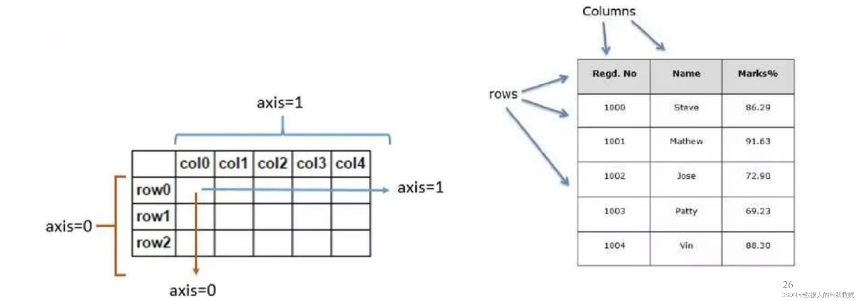
4.索引对象
pandas的索引对象负责管理轴标签和其他元数据(比如轴名称等)。
构建Series或DataFrame时,所用到的任何数组或其他序列的标签都会被转换成一个Index。
DataFrame行列,axis图解:
(1)显示DataFrame的索引和列
>>> df=pd.DataFrame(data,columns=['name','sex','year','city'],index=['a','b','c','d'])
>>> df
  name     sex  year city
a   张三  female  2001   北京
b   李四  female  2001   上海
c   王五    male  2003   广州
d   小明    male  2002   北京
>>> df.index
Index(['a', 'b', 'c', 'd'], dtype='object')
>>> print(df.columns)
Index(['name', 'sex', 'year', 'city'], dtype='object')
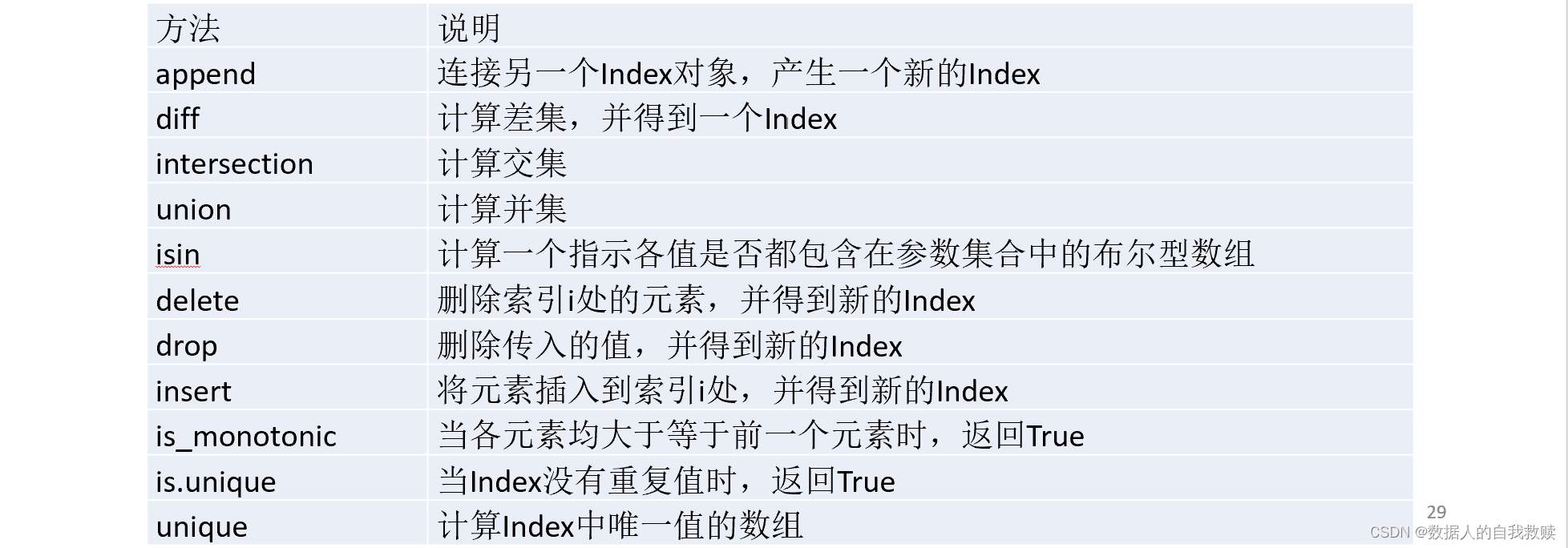
(2)对DataFrame的索引和列的测试
每个索引都有一些方法和属性,它们可用于设置逻辑并回答有关该索引所包含的数据的常见问题。Index的常用方法和属性见下表。
>>> df.index
Index(['a', 'b', 'c', 'd'], dtype='object')
>>> print(df.columns)
Index(['name', 'sex', 'year', 'city'], dtype='object')
>>> print('name' in df.columns)
True
>>> print('a' in df.index)
True
二、pandas索引操作
1.重新索引(Series)
索引对象是无法修改的,因此重新索引是指对索引重新排序而不是重新命名,如果某个索引值不存在的话,会引入缺失值。
对于重建索引引入的缺失值,可以利用fill_value参数填充。
>>> obj=pd.Series([7.2,-4.3,4.5,3.6],index=['b','a','d','c'])
>>> obj
b    7.2
a   -4.3
d    4.5
c    3.6
dtype: float64
>>> obj.reindex(['a','b','c','d','e'])
a   -4.3
b    7.2
c    3.6
d    4.5
e    NaN
dtype: float64
2.重新索引时填充缺失值(Series中)
对于顺序数据,比如时间序列,重新索引时可能需要进行插值或填值处理,利用参数method选项可以设置:
method='ffill'或'pad':表示前向值填充
method='bfill'或'backfill',表示后向值填充
>>> obj=pd.Series([7.2,-4.3,4.5,3.6],index=['b','a','d','c'])
>>> obj.reindex(['a','b','c','d','e'],fill_value=0)
a   -4.3
b    7.2
c    3.6
d    4.5
e    0.0
dtype: float64
3.缺失值的前后向填充(Series)
>>> import numpy as np
>>> obj=pd.Series(['blue','red','black'],index=[0,2,4])
>>> obj
0     blue
2      red
4    black
dtype: object
>>> obj.reindex(np.arange(6),method='ffill')
0     blue
1     blue
2      red
3      red
4    black
5    black
dtype: object
>>> obj.reindex(np.arange(6),method='backfill')
0     blue
1      red
2      red
3    black
4    black
5      NaN
dtype: object
4.重新索引(DateFrame中)
>>> import numpy as np
>>> import pandas as pd
>>> df4=pd.DataFrame(np.arange(9).reshape(3,3),index=['a','c','d'],columns=['one','two','four'])
>>> df4
   one  two  four
a    0    1     2
c    3    4     5
d    6    7     8
>>> df4.reindex(index=['a','b','c','d'],columns=['one','two','three','four'])
   one  two  three  four
a  0.0  1.0    NaN   2.0
b  NaN  NaN    NaN   NaN
c  3.0  4.0    NaN   5.0
d  6.0  7.0    NaN   8.0
5.重新索引, 传入fill_value=n填充缺失值(DateFrame中)
>>> df4.reindex(index=['a','b','c','d'],columns=['one','two','three','four'],fill_value=100)
   one  two  three  four
a    0    1    100     2
b  100  100    100   100
c    3    4    100     5
d    6    7    100     8
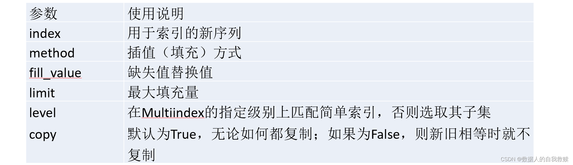
6.reindex函数参数
7.更换索引set_index函数
如果不希望使用默认的行索引,则可以在创建的时候通过index函数来设置。
在DateFrame数据中,如果希望将列数据作为索引,则可以通过set_index方法来实现。
>>> data={
...     'name':['张三','李四','王五','小明'],
...     'sex':['female','female','male','male'],
...     'year':[2001,2001,2003,2002],
...     'city':['北京','上海','广州','北京']
...     }
>>> df1=pd.DataFrame(data,columns=['name','year','sex','city'])
>>> df1
  name  year     sex city
0   张三  2001  female   北京
1   李四  2001  female   上海
2   王五  2003    male   广州
3   小明  2002    male   北京
>>> df5=df1.set_index('city')
>>> df5
     name  year     sex
city
北京     张三  2001  female
上海     李四  2001  female
广州     王五  2003    male
北京     小明  2002    male
三、DataFrame的数据查询与编辑
1.DataFrame的数据查询
在数据分析中,选取需要的数据进行分析处理是最基本的操作。在pandas中需要通过索引完成数据的选取。
(1)选取列
通过列索引或以属性的方式可以单独获取DataFrame的列数据,返回的数据类型为Series。
>>> df5
     name  year     sex
city
北京     张三  2001  female
上海     李四  2001  female
广州     王五  2003    male
北京     小明  2002    male
>>> w1=df5['name']
>>> print("选取1列数据:\n",w1)
选取1列数据:
 city
北京    张三
上海    李四
广州    王五
北京    小明
Name: name, dtype: object
>>> w2=df5[['name','year']]
>>> w2
     name  year
city
北京     张三  2001
上海     李四  2001
广州     王五  2003
北京     小明  2002
(2)选取行
通过切片形式可以选取一行或多行数据。
>>> print(df4)
   one  two  four
a    0    1     2
c    3    4     5
d    6    7     8
>>> print("显示前2行:\n",df4[:2])
显示前2行:
    one  two  four
a    0    1     2
c    3    4     5
>>> print("显示前2-3行:\n",df4[1:3])
显示前2-3行:
    one  two  four
c    3    4     5
d    6    7     8
(3)head,tail,sample方法选取行
选取通过DataFrame提供的head和tail方法可以得到多行数据,但是用这两种方法得到的数据都是从开始或者末尾获取连续的数据,而利用sample可以随机抽取数据并显示。

>>> df=pd.DataFrame(np.arange(100).reshape(20,5))
>>> df.head()    #前5行
    0   1   2   3   4
0   0   1   2   3   4
1   5   6   7   8   9
2  10  11  12  13  14
3  15  16  17  18  19
4  20  21  22  23  24
>>> df.head(3)    #前3行
    0   1   2   3   4
0   0   1   2   3   4
1   5   6   7   8   9
2  10  11  12  13  14
>>> df.tail()    #选尾5行
     0   1   2   3   4
15  75  76  77  78  79
16  80  81  82  83  84
17  85  86  87  88  89
18  90  91  92  93  94
19  95  96  97  98  99
>>> df.tail(3)    #选尾三行
     0   1   2   3   4
17  85  86  87  88  89
18  90  91  92  93  94
19  95  96  97  98  99
>>> df.sample(3)    #随机选3
    0   1   2   3   4
7  35  36  37  38  39
3  15  16  17  18  19
1   5   6   7   8   9
>>> df.nlargest(3,3)    #返回指定列最大的前三行
     0   1   2   3   4
19  95  96  97  98  99
18  90  91  92  93  94
17  85  86  87  88  89
(4)选取行和列

>>> print(df5.loc[:,['name','year']])    #显示name和year两列
     name  year
city
北京     张三  2001
上海     李四  2001
广州     王五  2003
北京     小明  2002
>>> print(df5.loc[['北京','上海'],['name','year']])    #显示北京和上海中的name和year两列
     name  year
city
北京     张三  2001
北京     小明  2002
上海     李四  2001
>>> print(df5.iloc[:2])    #用iloc选行与列,显示前两列
     name  year     sex
city
北京     张三  2001  female
上海     李四  2001  female
>>> print(df5.iloc[[1,3]])    #显示1、3行
     name  year     sex
city
上海     李四  2001  female
北京     小明  2002    male
>>> print(df5.iloc[[1,3],[1,2]])    #显示第一行1、2列元素和第三行1、2列元素
      year     sex
city
上海    2001  female
北京    2002    male
(5)布尔选择
可以对DateFrame中的数据进行布尔方式选择
>>> df5[df5['year']==2001]
     name  year     sex
city
北京     张三  2001  female
上海     李四  2001  female
2.DataFrame的数据的编辑
(1)增加数据
增加一行直接通过append方法传入字典结构数据即可。
>>> import pandas as pd
>>> data={
...     'name':['张三','李四','王五','小明'],
...     'sex':['female','female','male','male'],
...     'year':[2001,2001,2003,2002],
...     'city':['北京','上海','广州','北京']
...     }
>>> df=pd.DataFrame(data)
>>> data1={'city':'兰州','name':'李红','year':2005,'sex':'female'}
>>> df.append(data1,ignore_index=True)

Warning (from warnings module):
  File "<pyshell#43>", line 1
FutureWarning: The frame.append method is deprecated and will be removed from pandas in a future version. Use pandas.concat instead.
  name     sex  year city
0   张三  female  2001   北京
1   李四  female  2001   上海
2   王五    male  2003   广州
3   小明    male  2002   北京
4   李红  female  2005   兰州
增加列时,只需为要增加的列赋值即可创建一个新的列。
>>> df5['age']=20
>>> df5['C']=[85,78,96,80]
>>> df5
     name  year     sex  age   C
city
北京     张三  2001  female   20  85
上海     李四  2001  female   20  78
广州     王五  2003    male   20  96
北京     小明  2002    male   20  80
(2)删除数据
删除数据直接用drop方法,通过axis参数确定删除的是行/列。默认数据删除不修改原数据,需要在原数据删除行列时需要设置参数inplace=True。
>>>#删除数据行
>>> print(df5.drop('广州'))
     name  year     sex  age   C
city
北京     张三  2001  female   20  85
上海     李四  2001  female   20  78
北京     小明  2002    male   20  80
>>>#删除数据列
>>> print(df5.drop('age',axis=1,inplace=True))
None
>>>
>>> df5
     name  year     sex   C
city
北京     张三  2001  female  85
上海     李四  2001  female  78
广州     王五  2003    male  96
北京     小明  2002    male  80
(3)修改数据
修改数据时直接对选择的数据赋值即可。
需要注意的是,数据修改是直接对DataFrame数据修改,操作无法撤销,因此更改数据时要做好数据备份。
data
{'name': ['张三', '李四', '王五', '小明'], 'sex': ['female', 'female', 'male', 'male'], 'year': [2001, 2001, 2003, 2002], 'city': ['北京', '上海', '广州', '北京']}
df=pd.DataFrame(data)
df
  name     sex  year city
0   张三  female  2001   北京
1   李四  female  2001   上海
2   王五    male  2003   广州
3   小明    male  2002   北京
>>> df.iat[0,2]=2020    #修改指定行、列位置的数据值
>>> df.loc[:,'sex']=['male','female','male','female']    #修改某列的值
>>> df.loc[df['sex']=='female','year']=2050    #修改特定行的指定列
>>> df
  name     sex  year city
0   张三    male  2020   北京
1   李四  female  2050   上海
2   王五    male  2003   广州
3   小明  female  2050   北京
>>> df.replace('北京','武汉')    #把北京改成武汉
  name     sex  year city
0   张三    male  2020   武汉
1   李四  female  2050   上海
2   王五    male  2003   广州
3   小明  female  2050   武汉
>>> df    #原数据不变
  name     sex  year city
0   张三    male  2020   北京
1   李四  female  2050   上海
2   王五    male  2003   广州
3   小明  female  2050   北京
>>> df.replace(['张三','李四'],['赵六','赵八'])
  name     sex  year city
0   赵六    male  2020   北京
1   赵八  female  2050   上海
2   王五    male  2003   广州
3   小明  female  2050   北京
>>> df.replace({'王五':'赵七','小明':'赵九'})    #使用字典指定替换关系
  name     sex  year city
0   张三    male  2020   北京
1   李四  female  2050   上海
2   赵七    male  2003   广州
3   赵九  female  2050   北京
>>> df    #原数据不变
  name     sex  year city
0   张三    male  2020   北京
1   李四  female  2050   上海
2   王五    male  2003   广州
3   小明  female  2050   北京
四、pandas数据运算
1.算数运算
pandas的数据对象在进行算术运算时,如果有相同索引则进行算术运算,如果没有,则会自动进行数据对其,但会引入缺失值。
(1)series相加
>>> obj1=pd.Series([5.1,-2.6,7.8,10],index=['a','c','g','f'])
>>> obj1
a     5.1
c    -2.6
g     7.8
f    10.0
dtype: float64
>>> obj2=pd.Series([5.1,-2.6,7.8,10],index=['a','c','g','f'])
>>> obj2
a     5.1
c    -2.6
g     7.8
f    10.0
dtype: float64
>>> obj1+obj2
a    10.2
c    -5.2
g    15.6
f    20.0
dtype: float64
(2)DataFrame类型的数据相加
>>> a=np.arange(6).reshape(2,3)
>>> b=np.arange(4).reshape(2,2)
>>> a
array([[0, 1, 2],
       [3, 4, 5]])
>>> b
array([[0, 1],
       [2, 3]])
>>> df1=pd.DataFrame(a,columns=['a','b','e'],index=['A','C'])
>>> df1
   a  b  e
A  0  1  2
C  3  4  5
>>> df2=pd.DataFrame(b,columns=['a','b'],index=['A','D'])
>>> df2
   a  b
A  0  1
D  2  3
>>> df1+df2
     a    b   e
A  0.0  2.0 NaN
C  NaN  NaN NaN
D  NaN  NaN NaN
2.函数应用和映射
已定义好的函数可以通过以下三种方法应用到数据:
- map函数:将函数套用到Series的每个元素中
- apply函数:将函数套用到DataFrame的行/列上,行与列通过axis参数设置
- applymap函数,将函数套用到DataFrame的每个元素上
(1)将水果价格表中的“元”去掉
>>> data={'fruit':['apple','grape','banana'],'price':['30元','43元','28元']}
>>> df1=pd.DataFrame(data)
>>> df1
    fruit price
0   apple   30元
1   grape   43元
2  banana   28元
>>> def f(x):
...     return x.split('元')[0]
...
>>> '30元'.split('元')
['30', '']
>>> df1['price']=df1['price'].map(f)
>>> print('修改后的数据表:\n',df1)
修改后的数据表:
     fruit price
0   apple    30
1   grape    43
2  banana    28
(2)apply函数与applymap函数的使用方法
>>> df2=pd.DataFrame(np.random.randn(3,3),columns=['a','b','c'],index=['app','win','mac'])
>>> df2
            a         b         c
app -1.060500 -0.712209  0.779156
win  0.379755 -0.381884  0.695724
mac  0.606400  0.326212 -0.146500
>>> df2.apply(np.mean)
a   -0.024781
b   -0.255960
c    0.442793
dtype: float64
>>> df2
            a         b         c
app -1.060500 -0.712209  0.779156
win  0.379755 -0.381884  0.695724
mac  0.606400  0.326212 -0.146500
>>> df2.applymap(lambda x:'%.2f'%x)
         a      b      c
app  -1.06  -0.71   0.78
win   0.38  -0.38   0.70
mac   0.61   0.33  -0.15
3.排序
sort_index方法:对索引进行排序,默认为升序,降序排序时加参数ascending=False。
sort_values方法:对数值进行排序。by参数设置待排序的列名。
(1)Series的排序
>>> wy=pd.Series([1,-2,4,-4],index=['c','b','a','d'])
>>> wy
c    1
b   -2
a    4
d   -4
dtype: int64
>>> print('排序后的wy:\n',wy.sort_index())
排序后的wy:
 a    4
b   -2
c    1
d   -4
dtype: int64
>>> print('值排序后的wy:\n',wy.sort_values())
值排序后的wy:
 d   -4
b   -2
c    1
a    4
dtype: int64
(2)DataFrame的排序
对于DataFrame数据排序,通过指定轴方向,使用sort_index函数对行/列索引进行排序。如果要进行列排序,则通过sort_values函数把列名传给by参数即可。
>>> df=pd.DataFrame({'A':np.random.randint(1,100,4),
...                  'B':pd.date_range(start='20130101',periods=4,freq='D'),
...                  'C':pd.Series([1,2,3,4],index=['zhang','li','zhou','wang'],dtype='float32'),
...                  'D':np.array([3]*4,dtype='int32'),
...                  'E':pd.Categorical(["test","train","test","train"]),
...                  'F':'foo'})
>>> df
        A          B    C  D      E    F
zhang   5 2013-01-01  1.0  3   test  foo
li     87 2013-01-02  2.0  3  train  foo
zhou   15 2013-01-03  3.0  3   test  foo
wang   65 2013-01-04  4.0  3  train  foo
>>> df.sort_index(axis=0,ascending=False)    #对轴进行排序
        A          B    C  D      E    F
zhou   15 2013-01-03  3.0  3   test  foo
zhang   5 2013-01-01  1.0  3   test  foo
wang   65 2013-01-04  4.0  3  train  foo
li     87 2013-01-02  2.0  3  train  foo
>>> df.sort_index(axis=0,ascending=True)
        A          B    C  D      E    F
li     87 2013-01-02  2.0  3  train  foo
wang   65 2013-01-04  4.0  3  train  foo
zhang   5 2013-01-01  1.0  3   test  foo
zhou   15 2013-01-03  3.0  3   test  foo
>>> df.sort_index(axis=1,ascending=False)
         F      E  D    C          B   A
zhang  foo   test  3  1.0 2013-01-01   5
li     foo  train  3  2.0 2013-01-02  87
zhou   foo   test  3  3.0 2013-01-03  15
wang   foo  train  3  4.0 2013-01-04  65
>>> df.sort_values(by='A')    #对数据进行排序
        A          B    C  D      E    F
zhang   5 2013-01-01  1.0  3   test  foo
zhou   15 2013-01-03  3.0  3   test  foo
wang   65 2013-01-04  4.0  3  train  foo
li     87 2013-01-02  2.0  3  train  foo
>>> df
        A          B    C  D      E    F
zhang   5 2013-01-01  1.0  3   test  foo
li     87 2013-01-02  2.0  3  train  foo
zhou   15 2013-01-03  3.0  3   test  foo
wang   65 2013-01-04  4.0  3  train  foo
>>> dff=pd.DataFrame({'A':[3,8,3,9,3,10],'B':[4,1,8,2,6,3]})
>>> dff.sort_values(by=['A','B'],ascending=[True,False])    #A升序B降序
    A  B
2   3  8
4   3  6
0   3  4
1   8  1
3   9  2
5  10  3
4.汇总与统计
(1)数据汇总
在DataFrame中,可以通过sum方法对每列进行求和汇总,与Excel中的sum函数类似。如果设置axis=1指定轴方向,可以实现按行汇总。
- DataFrame中的汇总
>>> df2
            a         b         c
app -1.060500 -0.712209  0.779156
win  0.379755 -0.381884  0.695724
mac  0.606400  0.326212 -0.146500
>>> print('按列汇总:\n',df2.sum())
按列汇总:
 a   -0.074344
b   -0.767881
c    1.328379
dtype: float64
>>> print('按行汇总:\n',df2.sum(axis=1))
按行汇总:
 app   -0.993553
win    0.693595
mac    0.786112
dtype: float64
(2)描述与统计分析
利用describe方法对每个数值型的列数据进行统计。
>>> df2
a b c
app -1.060500 -0.712209 0.779156
win 0.379755 -0.381884 0.695724
mac 0.606400 0.326212 -0.146500
>>> df2.describe()
a b c
count 3.000000 3.000000 3.000000
mean -0.024781 -0.255960 0.442793
std 0.904089 0.530539 0.512045
min -1.060500 -0.712209 -0.146500
25% -0.340372 -0.547047 0.274612
50% 0.379755 -0.381884 0.695724
75% 0.493078 -0.027836 0.737440
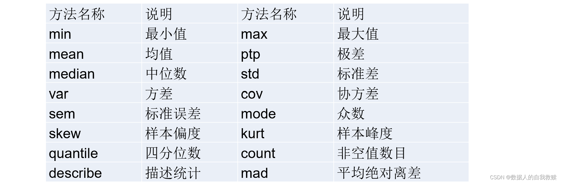
max 0.606400 0.326212 0.779156
pandas中常用的描述性统计量。
对于类别型特征的描述性统计,可以使用频数统计表。pandas库中通过unique方法获取不重复的数组,利用value_conuts方法实现频数统计。
>>> obj=pd.Series(['a','b','c','a','d','c'])
>>> obj.unique()
array(['a', 'b', 'c', 'd'], dtype=object)
>>> print(obj.unique())
['a' 'b' 'c' 'd']
>>> obj.value_counts()
a    2
c    2
b    1
d    1
dtype: int64