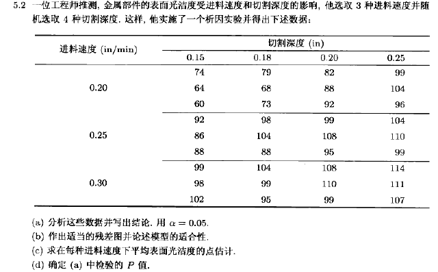
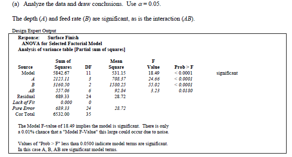
本文是实验设计与分析（第6版，Montgomery著，傅珏生译) 第5章析因设计引导5.7节思考题5.2 R语言解题。主要涉及方差分析，正态假设检验，残差分析，交互作用。

dataframe<-data.frame(

Surface=c(74,64,60,92,86,88,99,98,102,79,68,73,98,104,88,104,99,95,82,88,92,99,108,95,108,110,99,99,104,96,104,110,99,114,111,107),

Depth=gl(4, 9,36),

Feed=gl(3, 3, 36))

summary (dataframe)

dataframe.aov2 <- aov(Surface ~ Depth * Feed,data= dataframe)

summary (dataframe.aov2)

> summary (dataframe.aov2)

            Df Sum Sq Mean Sq F value   Pr(>F)   

Depth        3 2125.1   708.4  24.663 1.65e-07 ***

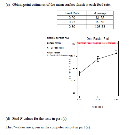
Feed         2 3160.5  1580.2  55.018 1.09e-09 ***

Depth:Feed   6  557.1    92.8   3.232    0.018 * 

Residuals   24  689.3    28.7                    

---

Signif. codes:  0 ‘***’ 0.001 ‘**’ 0.01 ‘*’ 0.05 ‘.’ 0.1 ‘ ’ 1

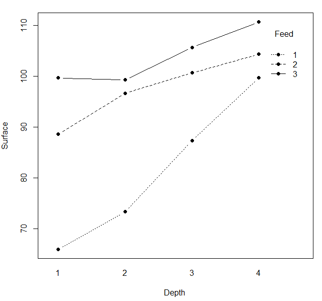
with(dataframe,interaction.plot(Depth, Feed, Surface,type="b",pch=19,fixed=T,xlab="Depth ",ylab=" Surface "))

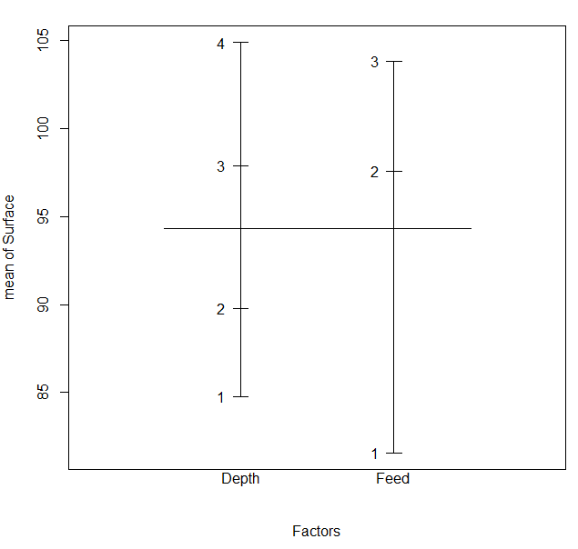
plot.design(Surface ~Depth* Feed,data= dataframe)

fit <-lm(Surface~Depth*Feed,data=dataframe)

anova(fit)

> anova(fit)

Analysis of Variance Table

Response: Surface

           Df  Sum Sq Mean Sq F value    Pr(>F)   

Depth       3 2125.11  708.37 24.6628 1.652e-07 ***

Feed        2 3160.50 1580.25 55.0184 1.086e-09 ***

Depth:Feed  6  557.06   92.84  3.2324   0.01797 * 

Residuals  24  689.33   28.72                     

---

Signif. codes:  0 ‘***’ 0.001 ‘**’ 0.01 ‘*’ 0.05 ‘.’ 0.1 ‘ ’ 1

summary(fit)

> summary(fit)

Call:

lm(formula = Surface ~ Depth * Feed, data = dataframe)

Residuals:

    Min      1Q  Median      3Q     Max

-8.6667 -3.6667 -0.3333  3.5833  8.0000

Coefficients:

             Estimate Std. Error t value Pr(>|t|)   

(Intercept)   66.0000     3.0942  21.330  < 2e-16 ***

Depth2         7.3333     4.3759   1.676  0.10675   

Depth3        21.3333     4.3759   4.875 5.70e-05 ***

Depth4        33.6667     4.3759   7.694 6.25e-08 ***

Feed2         22.6667     4.3759   5.180 2.64e-05 ***

Feed3         33.6667     4.3759   7.694 6.25e-08 ***

Depth2:Feed2   0.6667     6.1884   0.108  0.91511   

Depth3:Feed2  -9.3333     6.1884  -1.508  0.14456   

Depth4:Feed2 -18.0000     6.1884  -2.909  0.00770 **

Depth2:Feed3  -7.6667     6.1884  -1.239  0.22737   

Depth3:Feed3 -15.3333     6.1884  -2.478  0.02065 * 

Depth4:Feed3 -22.6667     6.1884  -3.663  0.00123 **

---

Signif. codes:  0 ‘***’ 0.001 ‘**’ 0.01 ‘*’ 0.05 ‘.’ 0.1 ‘ ’ 1

Residual standard error: 5.359 on 24 degrees of freedom

Multiple R-squared:  0.8945,    Adjusted R-squared:  0.8461

F-statistic: 18.49 on 11 and 24 DF,  p-value: 4.111e-09

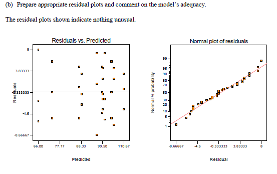
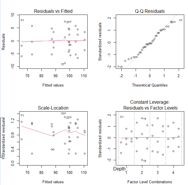
par(mfrow=c(2,2))

plot(fit)

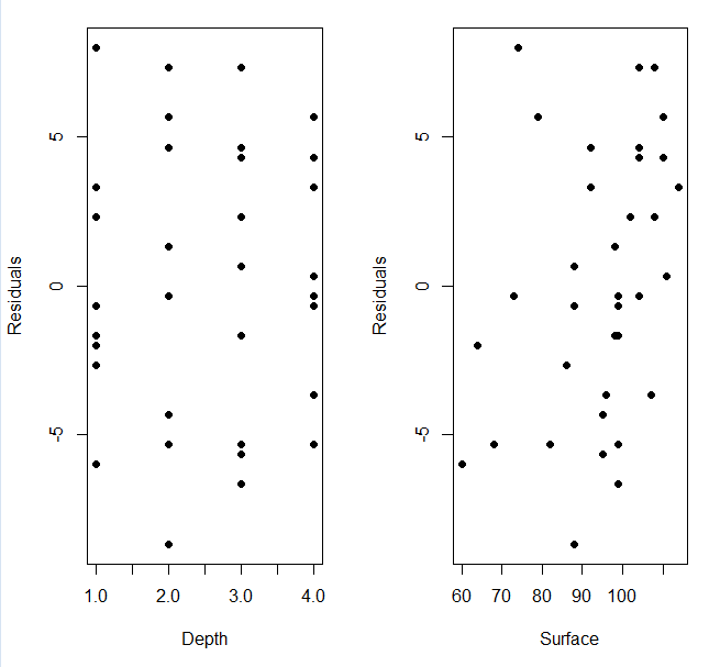
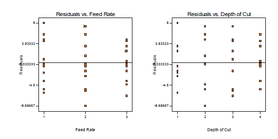
par(mfrow=c(1,2))

plot(as.numeric(dataframe$Depth), fit$residuals, xlab="Depth", ylab="Residuals", type="p", pch=16)

plot(as.numeric(dataframe$Surface), fit$residuals, xlab="Surface", ylab="Residuals", pch=16)