牛顿/莱布尼茨公式主要是为定积分的计算提供了高效的方法, 其主要含义在于求积分的函数($f(x)$)连续时候总是存在一条积分面积的函数($F(x)$)与之对应, 牛顿莱布尼茨公式吧微分和积分联系了起来, 提供了这种高效计算积分面积的方法

参考视频理解: https://www.bilibili.com/video/BV1qo4y1G7Da/

积分上限的函数及其导数

设函数$f(x)$在区间$[a,b]$上连续, 对于任意点$x\in [a,b]$, 函数$f(x)$在$[a,x]$上仍然连续, 定积分${\int }_a^{x}f(x)dx$一定存在. 此处的$x$即表示积分上限, 又表示积分变量, 因为积分值和变量名字无关, 又可以表示为${\int }_a^{x}f(t)dt$

如果上限$x$在区间$[a,b]$上任意变动, 对于每一个给定的$x$都有一个确定的值积分值与之对应, 所以在$[a,b]$上定义一个函数, 记做$\varphi (x)$, 那么$\varphi (x)={\int }_a^{x}f(t)dt$, $a\le x\le b$

函数$\varphi (x)$是积分上限$x$的函数, 也称为$f(t)$的变上限积分, $\varphi (x)$具有下面的性质

连续就可导, 导数等于原函数

如果函数$f(x)$在区间$[a,b]$上连续, 则积分上限函数$\varphi (x)={\int }_a^{x}f(t)dt$可导
${\varphi }^{\prime }(x)=\frac{d}{dx}{\int }_a^{x}f(t)dt=f(x)$, $a\le x\le b$

比如:
$$\frac{d}{dx}({\int }_a^{x}si{n}^{2}tdt)=si{n}^{2}x$$

原函数存在定理

如果函数$f(x)$在$[a,b]$上连续, 则函数$\varphi (x)={\int }_a^{x}f(t)dt$就是$f(x)$在$[a,b]$上的一个原函数

牛顿莱布尼茨公式

设函数$f(x)$在区间$[a,b]$上连续, $F(x)$是$f(x)$在$[a,b]$上的原函数, 则${\int }_a^{b}f(x)dx=F(b)-F(a)$

一个连续函数在区间上的定积分等于它的任意一个原函数在区间上的增量

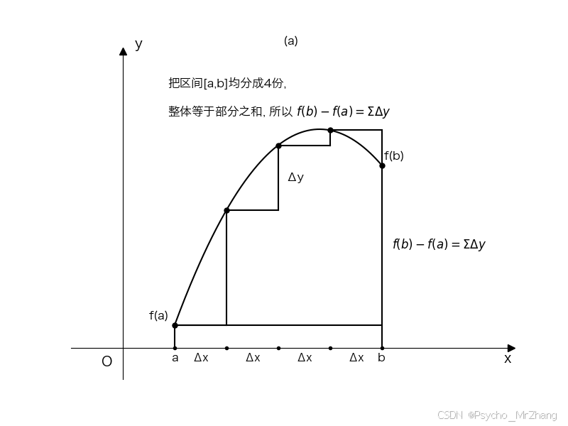
牛顿莱布尼茨公式几何解释

积分是在确定函数的导数的基础上, 通过一定的数学方法对原函数进行求解的过程. 积分的基本思想是通过微分的"无限求和"进行的. 微分是对原函数求导过程, 于是又可以讲积分看成微分逆向过程

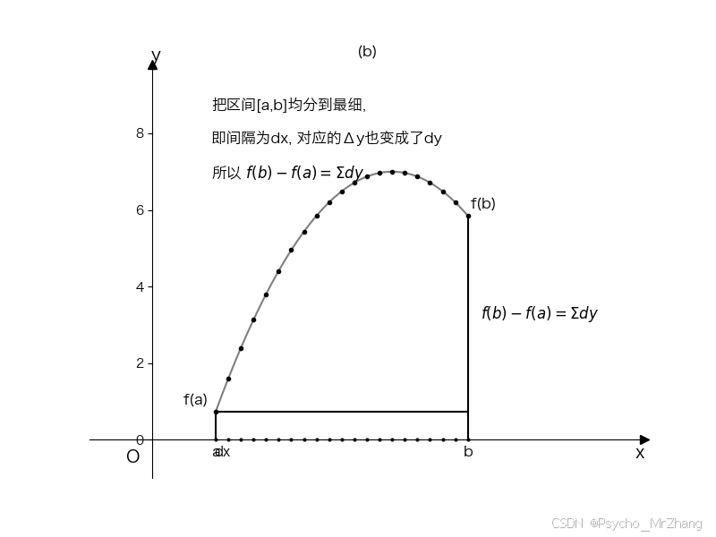
设函数$y=f(x)$, 吧区间$[a,b]$分为4份, 整体等于部分之和, $f(b)-f(a)=\sum \Delta y$,继续细分入图二表示, 间隔为$dx$, 对应的$\Delta y$变为了$dy$, 所以$f(b)-f(a)=\sum dy$, 从细分可知$dy=f^{\prime }(x)dx$, $f(b)-f(a)=\sum f^{\prime }(x)dx$

import numpy as np
import matplotlib.pyplot as plt


# 设置中文字体
plt.rcParams['font.sans-serif']=['Hiragino Sans GB'] # 修改字体
plt.rcParams['axes.unicode_minus'] = False # 正常显示负号



def func(x):
    return -0.8 * (x - 3.8)**2 + 7

# Define the interval [a, b]
a = 1.0
b = 5.0

# --- Plot 1 ---
n_plot1 = 4  # 4份
x_pts_plot1 = np.linspace(a, b, n_plot1 + 1)
y_pts_plot1 = func(x_pts_plot1)

x_curve = np.linspace(a, b, 200) # Smooth curve
y_curve = func(x_curve)

fig1, ax1 = plt.subplots(figsize=(8, 6))

# Plot the smooth curve
ax1.plot(x_curve, y_curve, 'k-')

# Plot the points on the curve
ax1.plot(x_pts_plot1, y_pts_plot1, 'ko', markersize=5)

# Set up axes (spines)
ax1.spines['left'].set_position('zero')
ax1.spines['bottom'].set_position('zero')
ax1.spines['right'].set_color('none')
ax1.spines['top'].set_color('none')
ax1.xaxis.set_ticks_position('bottom')
ax1.yaxis.set_ticks_position('left')

# Set plot limits (do this before placing arrows at ends of axes)
xlim1 = (-1, b + 2.5)
ylim1 = (-1, func(3.8) + 2.5) # func(3.8) is the peak
ax1.set_xlim(xlim1)
ax1.set_ylim(ylim1)

# Arrows for axes
ax1.plot(xlim1[1], 0, ">k", clip_on=False, markersize=7) # x-axis arrow
ax1.plot(0, ylim1[1], "^k", clip_on=False, markersize=7) # y-axis arrow

# Labels for axes
ax1.set_xlabel('x', loc='right', fontsize=14)
ax1.set_ylabel('y', loc='top', rotation=0, fontsize=14, labelpad=-20) # Adjust labelpad for y

# Origin 'O'
ax1.text(-0.2, -0.25, 'O', fontsize=14, ha='right', va='top')

# Vertical lines from x-axis to f(a) and f(b)
ax1.plot([a, a], [0, func(a)], 'k-')
ax1.plot([b, b], [0, func(b)], 'k-')

# X-axis ticks and labels
ax1.set_xticks([]) # Remove default ticks
ax1.text(a, -0.15, 'a', ha='center', va='top', fontsize=12)
ax1.text(b, -0.15, 'b', ha='center', va='top', fontsize=12)

# Plot points on x-axis for divisions and Δx labels
delta_x_val = (b - a) / n_plot1
for i in range(n_plot1):
    ax1.plot(x_pts_plot1[i], 0, 'ko', markersize=3)
    ax1.text(a + i * delta_x_val + delta_x_val / 2, -0.15, 'Δx', ha='center', va='top', fontsize=11)
ax1.plot(x_pts_plot1[n_plot1], 0, 'ko', markersize=3) # Last point 'b'

# Y-axis: remove default ticks
ax1.set_yticks([])

# Labels for f(a) and f(b)
ax1.text(a - 0.1, func(a) + 0.1, 'f(a)', ha='right', va='bottom', fontsize=12)
ax1.text(b + 0.05, func(b) + 0.1, 'f(b)', ha='left', va='bottom', fontsize=12)

# Horizontal line from (a, f(a)) to (b, f(a))
ax1.plot([a, b], [func(a), func(a)], 'k-')

# Step-like structure
for i in range(n_plot1):
    ax1.plot([x_pts_plot1[i], x_pts_plot1[i+1]], [y_pts_plot1[i], y_pts_plot1[i]], 'k-') # Horizontal
    ax1.plot([x_pts_plot1[i+1], x_pts_plot1[i+1]], [y_pts_plot1[i], y_pts_plot1[i+1]], 'k-') # Vertical

# Δy label (near the second step, as in image)
idx_delta_y = 1
x_mid_delta_y = x_pts_plot1[idx_delta_y+1] + 0.15
y_mid_delta_y = (y_pts_plot1[idx_delta_y] + y_pts_plot1[idx_delta_y+1]) / 2
ax1.text(x_mid_delta_y, y_mid_delta_y, 'Δy', ha='left', va='center', fontsize=12)

# Text annotations within the plot
text1_plot1 = "把区间[a,b]均分成4份,"
text2_plot1 = "整体等于部分之和, 所以 $f(b)-f(a) = \\Sigma \\Delta y$"
ax1.text(0.22, 0.92, text1_plot1, transform=ax1.transAxes, fontsize=12, ha='left', va='top')
ax1.text(0.22, 0.84, text2_plot1, transform=ax1.transAxes, fontsize=12, ha='left', va='top')

# Equation label on the right
y_center_sum_label_plot1 = (func(a) + func(b)) / 2
ax1.text(b + 0.2, y_center_sum_label_plot1, '$f(b)-f(a) = \\Sigma \\Delta y$', ha='left', va='center', fontsize=12)

plt.title("(a)") # Optional title for clarity
plt.show()


# --- Plot 2 ---
n_plot2 = 20  # "均分到最细" (many divisions)
x_pts_plot2 = np.linspace(a, b, n_plot2 + 1)
y_pts_plot2 = func(x_pts_plot2)

fig2, ax2 = plt.subplots(figsize=(8, 6))

# Plot the smooth curve (as a guide, points will be dominant)
ax2.plot(x_curve, y_curve, 'k-', alpha=0.5) # Lighter or thinner if needed

# Plot the many points on the curve
ax2.plot(x_pts_plot2, y_pts_plot2, 'ko', markersize=3) # Smaller dots

# Set up axes (spines)
ax2.spines['left'].set_position('zero')
ax2.spines['bottom'].set_position('zero')
ax2.spines['right'].set_color('none')
ax2.spines['top'].set_color('none')
ax2.xaxis.set_ticks_position('bottom')
ax2.yaxis.set_ticks_position('left')

# Set plot limits
xlim2 = (-1, b + 2.8) # Slightly more space for label on right
ylim2 = (-1, func(3.8) + 2.8)
ax2.set_xlim(xlim2)
ax2.set_ylim(ylim2)

# Arrows for axes
ax2.plot(xlim2[1], 0, ">k", clip_on=False, markersize=7)
ax2.plot(0, ylim2[1], "^k", clip_on=False, markersize=7)

# Labels for axes
ax2.set_xlabel('x', loc='right', fontsize=14)
ax2.set_ylabel('y', loc='top', rotation=0, fontsize=14, labelpad=-20)

# Origin 'O'
ax2.text(-0.2, -0.25, 'O', fontsize=14, ha='right', va='top')

# Vertical lines from x-axis to f(a) and f(b)
ax2.plot([a, a], [0, func(a)], 'k-')
ax2.plot([b, b], [0, func(b)], 'k-')

# X-axis ticks and labels 'a', 'b'
ax2.set_xticks([])
ax2.text(a, -0.15, 'a', ha='center', va='top', fontsize=12)
ax2.text(b, -0.15, 'b', ha='center', va='top', fontsize=12)

# dx representation on x-axis (many small dots)
for x_val in x_pts_plot2:
    ax2.plot(x_val, 0, 'ko', markersize=2)

# Label for 'dx' below the x-axis (first interval)
dx_val_plot2 = (b-a)/n_plot2
ax2.text(a + dx_val_plot2 / 2, -0.15, 'dx', ha='center', va='top', fontsize=11)

# Labels for f(a) and f(b)
ax2.text(a - 0.1, func(a) + 0.1, 'f(a)', ha='right', va='bottom', fontsize=12)
ax2.text(b + 0.05, func(b) + 0.1, 'f(b)', ha='left', va='bottom', fontsize=12)

# Horizontal line from (a, f(a)) to (b, f(a))
ax2.plot([a, b], [func(a), func(a)], 'k-')

# Text annotations within the plot
text1_plot2 = "把区间[a,b]均分到最细,"
text2_plot2 = "即间隔为dx, 对应的Δy也变成了dy"
text3_plot2 = "所以 $f(b)-f(a) = \\Sigma dy$"
ax2.text(0.22, 0.92, text1_plot2, transform=ax2.transAxes, fontsize=12, ha='left', va='top')
ax2.text(0.22, 0.84, text2_plot2, transform=ax2.transAxes, fontsize=12, ha='left', va='top')
ax2.text(0.22, 0.76, text3_plot2, transform=ax2.transAxes, fontsize=12, ha='left', va='top')

# Equation label on the right
y_center_sum_label_plot2 = (func(a) + func(b)) / 2
ax2.text(b + 0.2, y_center_sum_label_plot2, '$f(b)-f(a) = \\Sigma dy$', ha='left', va='center', fontsize=12)

plt.title("(b)") # Optional title
plt.show()

通俗的表示牛顿莱布尼茨公式的意义
$${\int }_a^{b}f(x)dx=f(\xi )(b-a)=F^{\prime }(\xi )(b-a)=F(b)-F(a)$$
积分中值定理: ${\int }_a^{b}f(x)dx=f(\xi )(b-a)$
微分中值定理: $F^{\prime }(\xi )(b-a)=F(b)-F(a)$

小试牛刀

1. 求${\int }_0^{\frac{\pi }{2}}(2cosx+sinx-1)dx$
   解: $=[2sinx-cosx-x{]}_0^{\frac{\pi }{2}}=3-\frac{\pi }{2}$

2. 设$f(x)=\{\begin{array}{l}2x,0\le x\le 1\\ 5,1<x\le 2\end{array}$, 求${\int }_0^{2}f(x)dx$
   解: $={\int }_0^{1}2xdx+{\int }_1^{2}5dx=x^2{|}_0^1+5x{|}_1^2=1+5=6$

Python求定积分

机器解定积分思想

牛顿莱布尼茨公式${\int }_a^{b}f(x)dx=F(b)-F(a)$求定积分的值, 不论在理论还是实际都具有重要的作用, 但是不能解决所有问题, 例如被积函数的原函数很难用初等函数表达, 或者原函数表达式过于复杂, 导致了这种方式的局限性, 机器积分求解过程可以分为下面几个步骤, 根据${\int }_a^{b}f(x)dx={\lim }_{\lambda \to 0}{\sum }_{i=1}^{n}f({\xi }_i)\Delta x_i$

1. 分割, $a=x_0<x_1<x_2<...<x_n=b$
2. 近似, $\Delta S_i\approx f(x{i}_i)\Delta x_i$, ${\xi }_i\in [x_{i-1},x_i]$, $\Delta x_i=x_i-x_{i-1},i=1,2,...,n$
3. 求和, ${\sum }_{i=1}^{n}f({\xi }_i)\Delta x_i$
4. 求极限, ${\lim }_{\lambda \to 0}{\sum }_{i=1}^{n}f({\xi }_i)\Delta x_i$

求解过程为计算机求解提供思路, 将求解区间分为$n$份, 步长为$\frac{b-a}{n}$, 循环$n$次求解$n$个小梯形的面积之和就是定积分近似解

牛刀小试

编写程序求${\int }_0^2{x}^{2}dx$

import numpy as np
from scipy.integrate import dblquad

def func(x):
    # np.exp 为 e 的指定次幂
    return x ** 2


def trape(func, n, a, b):
    """
    :param func: 原函数
    :param n: 分为多少份计算
    :param a: 积分下限
    :param b: 积分上限
    :return:
    """
    # 计算步长
    h = (b - a) / n
    sum = 0
    for i in range(1, n + 1):
        x0 = a + (i - 1) * h # 计算第i个梯形的底边x0
        x1 = a + i * h  # 计算第i个梯形的顶边x1
        # 计算梯形面积 (底边(y=f(x0)) + 顶边y=f(x1)) * h /2
        sum += (func(x0) + func(x1)) * h / 2

    return sum



print(trape(func, 2, 0, 3))
# 10.125
print(trape(func, 20, 0, 3))
# 9.01125
print(trape(func, 200, 0, 3))
# 9.0001125
print(trape(func, 2000, 0, 3))
# 9.000001125000004
print(trape(func, 20000, 0, 3))
# 9.000000011250007
print(trape(func, 200000, 0, 3))
# 9.000000000112504

函数介绍

quad

入参

• func: 积分函数
• a: 积分下限
• b: 积分上限

出参

• 积分值
• 误差

dblquad

入参

• func: 积分函数
• a: x的下限
• b: x的上限
• gfun: 变量y的下限
• hfun: 变量y的上限

出参

• 积分值
• 误差

题目列表

1. 求${\int }_0^{3}co{s}^2(e^x)dx$

import numpy as np
from scipy.integrate import quad


def func(x):
    # np.exp 为 e 的指定次幂
    return np.cos(np.e ** x) ** 2


print(quad(func, 0, 3))

"""output:
积分值, 误差
(1.296467785724373, 1.3977970832667816e-09)
"""

2. 求$\int {\int }_x^y{e}^{-x^2-y^2}dxdy$, 其中$D=\{(x,y)|0\le x\le 10,0\le y\le 10\}$

import numpy as np
from scipy.integrate import dblquad


def func(x, y):
    # np.exp 为 e 的指定次幂
    return np.exp(-x** 2 - y ** 2)

x_a = 0
x_b = 10
y_a = 0
y_b = 10

print(dblquad(func, x_a, x_b, lambda y: y_a, lambda y: y_b))

"""output:
积分值, 误差
(0.7853981633974476, 1.3753098510206357e-08)
"""