征程 6 yolov5s-rgb-nhwc 量化指南

在征程 6 平台，我们可以按照这个方式编译 input_typr_rt 为 rgb，且 layout 为 NHWC 的模型。这样做的好处是，当用户的数据输入源本身就是 NHWC 的 rgb 图像时，这么做可以避免额外的数据处理操作。这里以 yolov5s 为例进行介绍。

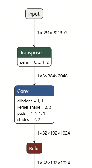
一、模型信息

输入节点

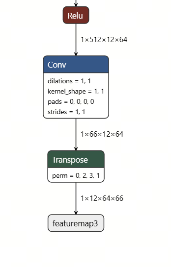
输出节点（其中一个）

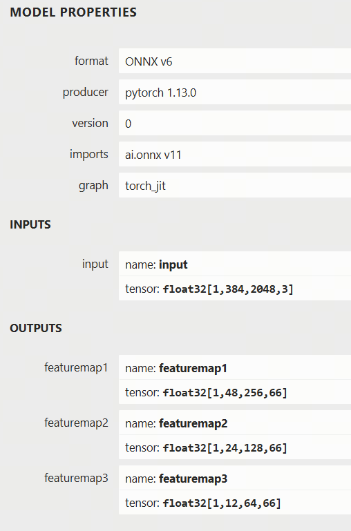
输入输出信息总览

二、校准数据

seed100 文件夹存放原始图像，可借助 horizon_model_convert_sample 的脚本完成校准数据的处理。

02_preprocess.sh 脚本内容如下：

set -e -v
cd 
$(dirname $
0) || exit
python3 ../../data_preprocess.py \
  --src_dir ./seed100 \
  --dst_dir ./calibration_data_rgb_f32 \
  --pic_ext .rgb \
  --read_mode opencv \
  --saved_data_type float32

preprocess.py 脚本相关内容修改如下：

from horizon_tc_ui.data.transformer import (PadResizeTransformer,
                                            BGR2RGBTransformer,
                                            NormalizeTransformer)
def calibration_transformers():
    transformers = [
        PadResizeTransformer(target_size=(384, 2048)),
        BGR2RGBTransformer(data_format="HWC"),
        NormalizeTransformer(255.0)
    ]
    return transformers

这段代码的主要作用是创建一个由多个数据预处理步骤组成的转换器（transformers）列表。这些转换器会对输入数据进行处理，以适应深度学习模型的要求。

PadResizeTransformer：这个转换器的作用是对输入数据进行填充（padding）和调整大小（resize），通常是为了确保输入的图像尺寸与模型要求的输入尺寸一致。
BGR2RGBTransformer：这个转换器将输入图像从 BGR 格式转换为 RGB 格式。BGR 是 OpenCV 默认的颜色格式，而许多深度学习框架（如 TensorFlow 或 PyTorch）更习惯使用 RGB 格式。因此，这个转换器是为了进行格式的转换。
NormalizeTransformer：这个转换器用于对图像进行归一化处理，将像素值缩放到指定的范围。归一化是深度学习中常见的预处理步骤，有助于提高模型的收敛速度和性能。

这段代码的作用是定义并返回一个包含多个数据预处理步骤的转换器列表。这些预处理步骤包括：

填充和调整大小：将图像调整为目标尺寸 (384, 2048)。
颜色格式转换：将图像从 BGR 格式转换为 RGB 格式。
归一化：将图像像素值缩放到 0 到 1 的范围内。

这些步骤通常用于图像数据预处理，以便将原始图像调整为模型输入所需要的格式和数值范围。

三、YAML

calibration_parameters:
  cal_data_dir: "./calibration_data_rgb_f32"
  quant_config: {
    "model_config": {
      "all_node_type": "int8",
      "activation": {
        "calibration_type": "max",
        "max_percentile": 0.99999,
      },
    },
  }  
compiler_parameters:
  compile_mode: latency
  debug: true
  jobs: 32
  optimize_level: O2
input_parameters:
  input_name: input
  input_shape: 1x384x2048x3
  input_layout_rt: NHWC
  input_layout_train: NHWC
  input_type_rt: rgb
  input_type_train: rgb
  std_value: 255.0
model_parameters:
  march: nash-m
  onnx_model: ./yolov5s.onnx
  output_model_file_prefix: yolov5s
  working_dir: ./model_output

四、模型编译

hb_compile -c ./config.yaml
+-------------+-------------------+------------------+
| TensorName  | Calibrated Cosine | Quantized Cosine |
+-------------+-------------------+------------------+
| featuremap1 | 0.999015          | 0.998999         |
| featuremap2 | 0.999408          | 0.999395         |
| featuremap3 | 0.999311          | 0.999321         |
+-------------+-------------------+------------------+

五、python 推理

import cv2
import numpy as np
from horizon_tc_ui.hb_runtime import HBRuntime
def prepare_onnx_input():
    data = cv2.imread('./seed.jpg').astype(np.float32)
    data = cv2.cvtColor(data, cv2.COLOR_BGR2RGB)
    data = data / 255.0
    data = data[np.newaxis,:,:,:]
    return data
def prepare_bc_input():
    data = cv2.imread('./seed.jpg').astype(np.uint8)
    data = cv2.cvtColor(data, cv2.COLOR_BGR2RGB)
    data = (data - 128).astype(np.int8)
    data = data[np.newaxis,:,:,:]
    return data
def infer_onnx():
    data = prepare_onnx_input()
    sess = HBRuntime("yolov5s.onnx")
    input_names = sess.input_names
    output_names = sess.output_names
    input_feed = {input_names[0]: data}
    output = sess.run(output_names, input_feed)
    print("==========infer_onnx==========")
    print(output[0][0][0][0])
    return 0
def infer_ori_onnx():
    data = prepare_onnx_input()
    sess = HBRuntime("./model_output/yolov5s_original_float_model.onnx")
    input_names = sess.input_names
    output_names = sess.output_names
    input_feed = {input_names[0]: data}
    output = sess.run(output_names, input_feed)
    print("==========infer_ori_onnx==========")
    print(output[0][0][0][0])
def infer_opt_onnx():
    data = prepare_onnx_input()
    sess = HBRuntime("./model_output/yolov5s_optimized_float_model.onnx")
    input_names = sess.input_names
    output_names = sess.output_names
    input_feed = {input_names[0]: data}
    output = sess.run(output_names, input_feed)
    print("==========infer_opt_onnx==========")
    print(output[0][0][0][0])
def infer_calib_onnx():
    data = prepare_onnx_input()
    sess = HBRuntime("./model_output/yolov5s_calibrated_model.onnx")
    input_names = sess.input_names
    output_names = sess.output_names
    input_feed = {input_names[0]: data}
    output = sess.run(output_names, input_feed)
    print("==========infer_calib_onnx==========")
    print(output[0][0][0][0])
def infer_ptq_onnx():
    data = prepare_onnx_input()
    sess = HBRuntime("./model_output/yolov5s_ptq_model.onnx")
    input_names = sess.input_names
    output_names = sess.output_names
    input_feed = {input_names[0]: data}
    output = sess.run(output_names, input_feed)
    print("==========infer_ptq_onnx==========")
    print(output[0][0][0][0])
def infer_quantized_bc():
    data = prepare_bc_input()
    sess = HBRuntime("./model_output/yolov5s_quantized_model.bc")
    input_names = sess.input_names
    output_names = sess.output_names
    input_feed = {input_names[0]: data}
    output = sess.run(output_names, input_feed)
    print("==========infer_quantized_bc==========")
    print(output[0][0][0][0])
if 
name
 == "
__main__
":
    infer_onnx()
    infer_ori_onnx()
    infer_opt_onnx()
    infer_calib_onnx()
    infer_ptq_onnx()
    infer_quantized_bc()

这段代码的主要作用是使用不同的模型和输入数据进行推理（inference），并输出推理结果。它通过调用 HBRuntime 来加载不同的模型进行推理。下面是对代码的详细分析：

1.导入必要的库：

cv2：用于图像处理，加载和转换图像。
numpy：用于数值计算，尤其是矩阵操作。
HBRuntime：从 horizon_tc_ui.hb_runtime 导入，显然是一个用于执行推理任务的接口，可能是用于调用经过优化的计算图或深度学习模型。

2.准备输入数据：

prepare_onnx_input()：该函数读取图像文件 seed.jpg，将其转换为 RGB 格式，进行归一化处理，并为模型的输入格式添加额外的维度（np.newaxis）。数据被归一化到 [0, 1] 范围，以便于输入 ONNX 模型。
prepare_bc_input()：此函数和 prepare_onnx_input() 类似，不过它读取的图像经过不同的处理。图像被转换为 np.uint8 类型，减去 128 后转换为 np.int8 类型，这通常是用于处理量化后的模型数据格式。

3.进行推理的不同函数：

每个 infer_*_onnx 或 infer_quantized_bc 函数负责加载不同的模型并执行推理：
- infer_onnx()：加载 yolov5s.onnx 模型并进行推理。
- infer_ori_onnx()：加载原始浮点数版本的 yolov5s 模型（yolov5s_original_float_model.onnx）。
- infer_opt_onnx()：加载优化过的浮点数版本的 yolov5s 模型（yolov5s_optimized_float_model.onnx）。
- infer_calib_onnx()：加载经过校准的浮点数模型（yolov5s_calibrated_model.onnx）。
- infer_ptq_onnx()：加载经过量化后的浮点数模型（yolov5s_ptq_model.onnx）。
- infer_quantized_bc()：加载量化后的 BC 格式模型（yolov5s_quantized_model.bc）。

4.推理过程：

每个 infer_* 函数都会执行以下步骤：
- 调用相应的准备输入函数（如 prepare_onnx_input() 或 prepare_bc_input()），将图像转换为模型所需的输入格式。
- 使用 HBRuntime 加载不同的模型。
- 获取模型的输入和输出节点名称。
- 将输入数据传入模型进行推理。
- 输出推理结果的一部分（通过 output[0][0][0][0] 打印输出，可能是某个检测框的值）。

5.主函数 if name == "__main__":：

在主程序执行时，依次调用上述所有的推理函数进行推理，打印每个模型的推理结果。

六、总结：

这段代码主要用于进行不同版本的 YOLOv5 模型的推理，涉及到原始浮点数模型、优化后的浮点数模型、量化模型、校准模型等，并对每种模型进行推理结果输出。通过不同的输入准备函数，代码还演示了如何处理不同的数据格式（如浮点数和量化后的数据）。

输出信息如下，可以看到，数值大体相当，可以认为推理结果正确。

==========infer_onnx==========
[ -0.36140022   0.14068425  -0.12884808   0.38683856 -10.027128
  -3.727932    -2.6472187   -3.4907613   -0.8754431   -1.8876309
  -1.6180705   -2.6833398   -2.4786358   -3.0784476   -3.320454
  -4.3665814   -3.2660558   -3.767973    -4.428035    -3.4952142
  -2.8823838   -4.920804    -0.36190268   0.24379599  -0.52514255
  -0.40856832 -11.233256    -3.9329526   -2.7249336   -3.4358976
  -0.8108312   -1.852678    -1.4934196   -2.7427323   -2.4955802
  -3.2720697   -3.3685834   -4.5204425   -3.2479987   -3.8060267
  -4.4632807   -3.5123816   -2.8149266   -5.1647396   -0.35967097
   0.22670399  -0.854579    -0.18010648 -13.903754    -4.169511
  -2.4058053   -3.4251635   -0.8236269   -1.8188286   -1.6522415
  -2.8259125   -2.4029486   -3.3103113   -3.409004    -4.688325
  -3.2148345   -3.948554    -4.4465227   -3.5018692   -2.8768973  -5.213859  ]
==========infer_ori_onnx==========
[ -0.36140022   0.14068425  -0.12884808   0.38683856 -10.027128
  -3.727932    -2.6472187   -3.4907613   -0.8754431   -1.8876309
  -1.6180705   -2.6833398   -2.4786358   -3.0784476   -3.320454
  -4.3665814   -3.2660558   -3.767973    -4.428035    -3.4952142
  -2.8823838   -4.920804    -0.36190268   0.24379599  -0.52514255
  -0.40856832 -11.233256    -3.9329526   -2.7249336   -3.4358976
  -0.8108312   -1.852678    -1.4934196   -2.7427323   -2.4955802
  -3.2720697   -3.3685834   -4.5204425   -3.2479987   -3.8060267
  -4.4632807   -3.5123816   -2.8149266   -5.1647396   -0.35967097
   0.22670399  -0.854579    -0.18010648 -13.903754    -4.169511
  -2.4058053   -3.4251635   -0.8236269   -1.8188286   -1.6522415
  -2.8259125   -2.4029486   -3.3103113   -3.409004    -4.688325
  -3.2148345   -3.948554    -4.4465227   -3.5018692   -2.8768973  -5.213859  ]
==========infer_opt_onnx==========
[ -0.36140022   0.14068425  -0.12884808   0.38683856 -10.027128
  -3.727932    -2.6472187   -3.4907613   -0.8754431   -1.8876309
  -1.6180705   -2.6833398   -2.4786358   -3.0784476   -3.320454
  -4.3665814   -3.2660558   -3.767973    -4.428035    -3.4952142
  -2.8823838   -4.920804    -0.36190268   0.24379599  -0.52514255
  -0.40856832 -11.233256    -3.9329526   -2.7249336   -3.4358976
  -0.8108312   -1.852678    -1.4934196   -2.7427323   -2.4955802
  -3.2720697   -3.3685834   -4.5204425   -3.2479987   -3.8060267
  -4.4632807   -3.5123816   -2.8149266   -5.1647396   -0.35967097
   0.22670399  -0.854579    -0.18010648 -13.903754    -4.169511
  -2.4058053   -3.4251635   -0.8236269   -1.8188286   -1.6522415
  -2.8259125   -2.4029486   -3.3103113   -3.409004    -4.688325
  -3.2148345   -3.948554    -4.4465227   -3.5018692   -2.8768973  -5.213859  ]
==========infer_calib_onnx==========
[ -0.43238506   0.11002721  -0.07907629   0.40861583  -9.97794
  -3.6856174   -2.735222    -3.633584    -0.96581066  -1.6290709
  -1.5608525   -2.6134243   -2.3609822   -3.004236    -3.2058396
  -4.3830314   -3.0389607   -3.8800378   -4.4044924   -3.417421
  -2.7247229   -4.8871512   -0.41328928   0.18615645  -0.5093392
  -0.40168345 -11.165181    -3.8985913   -2.8401194   -3.6001463
  -0.93232083  -1.6206057   -1.4628205   -2.6981122   -2.3167949
  -3.2422874   -3.2519443   -4.5322804   -3.002402    -3.9381328
  -4.4415045   -3.4783902   -2.6498706   -5.107289    -0.43616575
   0.1885212   -0.8195747   -0.17303436 -13.778434    -4.1264076
  -2.5370815   -3.6029017   -0.91676974  -1.5773652   -1.6292106
  -2.8174675   -2.254434    -3.2408853   -3.2774894   -4.6843886
  -2.9586797   -4.0764017   -4.4135203   -3.4192595   -2.7116857  -5.1625004 ]
==========infer_ptq_onnx==========
[ -0.43238506   0.11002721  -0.07907629   0.40861583  -9.97794
  -3.6856174   -2.735222    -3.633584    -0.96581066  -1.6290709
  -1.5608525   -2.6134243   -2.3609822   -3.004236    -3.2058396
  -4.3830314   -3.0389607   -3.8800378   -4.4044924   -3.417421
  -2.7247229   -4.8871512   -0.41328928   0.18615645  -0.5093392
  -0.40168345 -11.165181    -3.8985913   -2.8401194   -3.6001463
  -0.93232083  -1.6206057   -1.4628205   -2.6981122   -2.3167949
  -3.2422874   -3.2519443   -4.5322804   -3.002402    -3.9381328
  -4.4415045   -3.4783902   -2.6498706   -5.107289    -0.43616575
   0.1885212   -0.8195747   -0.17303436 -13.778434    -4.1264076
  -2.5370815   -3.6029017   -0.91676974  -1.5773652   -1.6292106
  -2.8174675   -2.254434    -3.2408853   -3.2774894   -4.6843886
  -2.9586797   -4.0764017   -4.4135203   -3.4192595   -2.7116857  -5.1625004 ]
==========infer_quantized_bc==========
[ -0.37202302   0.18693314  -0.06567554   0.40963683  -9.98054
  -3.6307201   -2.703453    -3.4887328   -0.9094247   -1.7791512
  -1.54388     -2.5430217   -2.399686    -2.996389    -3.1917665
  -4.3041177   -2.9921875   -3.7818878   -4.3069286   -3.3589668
  -2.8220906   -4.8398676   -0.34859642   0.2652311   -0.50713307
  -0.40864512 -10.916675    -3.8250697   -2.8117514   -3.4346225
  -0.8636422   -1.7796087   -1.4381862   -2.6121027   -2.3534453
  -3.2200432   -3.2179508   -4.427741    -2.9437149   -3.8163087
  -4.323068    -3.4090939   -2.7401025   -5.0440025   -0.37643808
   0.2674079   -0.8191366   -0.1740098  -13.797277    -4.0533657
  -2.4911644   -3.4408677   -0.8496779   -1.7336257   -1.605081
  -2.7330828   -2.2852495   -3.2210054   -3.2354999   -4.5808883
  -2.8986108   -3.9594183   -4.282491    -3.3463652   -2.8071992  -5.093343  ]

-4.323068 -3.4090939 -2.7401025 -5.0440025 -0.37643808
0.2674079 -0.8191366 -0.1740098 -13.797277 -4.0533657
-2.4911644 -3.4408677 -0.8496779 -1.7336257 -1.605081
-2.7330828 -2.2852495 -3.2210054 -3.2354999 -4.5808883
-2.8986108 -3.9594183 -4.282491 -3.3463652 -2.8071992 -5.093343 ]


 至此，模型的量化和 python 推理验证就结束了。我们可以愉快地开始 C++推理了