马上要参加亚太杯啦，听说今年亚太杯有经典的物理题，没什么好说的，盘它！
偏微分方程的数值解十分重要

椭圆型偏微分方程（不含时）

数值解法

$u_{i,j}=\frac{u_{i,j-1}+u_{i-1,j}+u_{i+1,j}+u_{i,j+1}-h^2f(x,y)}{4}$

二维拉普拉斯方程

$\frac{\partial^2u(x,y)}{\partial^2 x}+\frac{\partial^2u(x,y)}{\partial^2 y}=0$

例

边界条件

$\left\{\begin{matrix} \frac{log(1+i)}{10}&\,\,(x_{-1},y_i) \\ sin(\frac{2\pi i}{(M-1)})&\,\,(x_0,y_i) \\ cos(i)&\,\, (x_i,y_{-1}))\\ e^{\frac{i}{100}} & \,\,(x_i,y_0) \end{matrix}\right.$

import numpy as np
import matplotlib.pyplot as plt
from mpl_toolkits.mplot3d import Axes3D
from matplotlib import cm
import math

limit = 1000 #迭代次数极限
N = 101 #X轴方向分割次数
M = 101 #Y轴方向分割次数

def iteration(u):
    global N
    global M
    u_next = np.zeros((M,N))
    for i in range(1,N-1):
        for j in range(1,M-1):
            u_next[i][j] = 0.25*(u[i][j-1]+u[i-1][j]+u[i+1][j]+u[i][j+1])
    for i in range(1,N-1):
        for j in range(1,M-1):
            u[i][j] = u_next[i][j]

u = np.zeros((M,N))
for i in range(M):
    u[0][i] = math.sin(2*math.pi*i/(M-1))
for i in range(N):
    u[-1][i] = math.log(1+i)/10
for i in range(M):
    u[i][-1] = math.cos(i)
for i in range(N):
    u[i][0] = math.e ** (i/100)
for i in range(limit):
    iteration(u)

x = np.arange(0,N)
y = np.arange(0,M)
X,Y = np.meshgrid(x,y)
fig = plt.figure()
ax = Axes3D(fig)
ax.plot_wireframe(X,Y,u)
plt.show()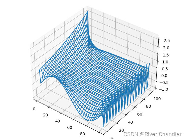

二维泊松方程

$\frac{\partial^2u(x,y)}{\partial^2 x}+\frac{\partial^2u(x,y)}{\partial^2 y}=f(x,y)$

例

$f(x,y)=x+y$

边界条件： $\left\{\begin{matrix} \frac{log(1+i)}{10}&\,\,(x_{-1},y_i) \\ sin(\frac{2\pi i}{(M-1)})&\,\,(x_0,y_i) \\ cos(i)&\,\, (x_i,y_{-1}))\\ e^{\frac{i}{100}} & \,\,(x_i,y_0) \end{matrix}\right.$

import numpy as np
import matplotlib.pyplot as plt
from mpl_toolkits.mplot3d import Axes3D
from matplotlib import cm
import math

limit = 1000 #迭代次数极限
N = 101 #X轴方向分割次数
M = 101 #Y轴方向分割次数
h = 1
f = lambda x,y : x+y

def iteration(u):
    global N
    global M
    u_next = np.zeros((M,N))
    for i in range(1,N-1):
        for j in range(1,M-1):
            u_next[i][j] = 0.25*(u[i][j-1]+u[i-1][j]+u[i+1][j]+u[i][j+1]-h**2*f(i,j))
    for i in range(1,N-1):
        for j in range(1,M-1):
            u[i][j] = u_next[i][j]

u = np.zeros((M,N))
for i in range(M):
    u[0][i] = math.sin(2*math.pi*i/(M-1))
for i in range(N):
    u[-1][i] = math.log(1+i)/10
for i in range(M):
    u[i][-1] = math.cos(i)
for i in range(N):
    u[i][0] = math.e ** (i/100)
for i in range(limit):
    iteration(u)

x = np.arange(0,N)
y = np.arange(0,M)
X,Y = np.meshgrid(x,y)
fig = plt.figure()
ax = Axes3D(fig)
ax.plot_wireframe(X,Y,u)
plt.show()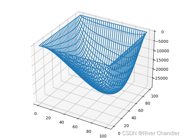

二阶抛物型偏微分方程

一维热传导方程

$\frac{\partial u(x,t)}{\partial t}=\lambda \frac{\partial^2 u(x,t)}{\partial x^2}\,\,\,0\leq t \leq T,0\leq x \leq l$

边界条件： $\left\{\begin{matrix} u(x,0)=f(x)\\ u(0,t)=g_1(t)\\ u(l,t)=g_2(t) \end{matrix}\right.$

空间步长 $h$ 与时间步长 $\tau$

递推关系： $\left\{\begin{matrix} u_{i,k+1}=\frac{\lambda \tau}{h^2}u_{i+1,k}+(1-2\frac{\lambda \tau}{h^2})u_{i,k}+\frac{\lambda \tau}{h^2}u_{i-1,k}\\ u_{i,0}=f(ih)\,\,\, i=1,2,...,N-1,N=\frac{l}{h}\\ u_{0,k}=g_1(k\tau)\,\,\, k=0,1,...,M,M=\frac{T}{\tau}\\ u_{N,k}=g_2(k\tau) \end{matrix}\right.$

例：

import numpy as np
import matplotlib.pyplot as plt

#参量设置
l = 1
lambde =     1.0
start_time = 0.0
end_time =   10
h =   0.05
tau = 0.001
K = lambde  * tau /h**2
#参量设置结束

#数值解向量
U = np.zeros((int((l)/h),int((end_time-start_time)/tau)))
#数值解向量组设置结束


#边界条件设置
for j in range(int((end_time-start_time)/tau)):
    U[0,j] = np.sin(j)
    U[-1,j] = 0.0
#边界条件设置结束


#初始条件设置
for i in range(int(l/h)):
    U[i,0] = 0
#初始条件设置结束



#时域差分法
for j in range(int((end_time-start_time)/tau)-1):
    for i in range(1,int(l/h)-1):
        try:
            U[i,j+1] = K*U[i+1,j]+(1-2*K)*U[i,j]+K*U[i-1,j]
        except:
            print("i,j",i," ",j)
#时域差分法设置结束


#数据可视化
for i in range(10):
    try:
        u = U[:,i*1000]
        plt.plot(range(len(u)),u)
        plt.pause(0.5)
    except:
        print("超出时域范围")

for i in range(20):
    try:
        u = U[i,:]
        plt.plot(range(len(u)),u)
        plt.pause(0.5)
    except:
        print("超出长度范围")

二维热传导方程

$\frac{\partial u}{\partial t}=\lambda (\frac{\partial ^2 u}{\partial x^2}+\frac{\partial ^2 u}{\partial y^2})+q_v\,\,\, 0\leq t \leq t_e,0<x<1,0<y<1$

边界条件： $\left\{\begin{matrix} u(x,y,0)=u_0(x,y)\\ u(0,y,t)=u_a(t)\\ u(1,y,t)=u_b(t)\\ u(x,0,t)=u_c(t)\\ u(x,1,t)=u_d(t)\\ \end{matrix}\right.$

递推关系： $\left\{\begin{matrix} u_{i,j}^{k+1}=r_x(u_{i-1,j}^{k}+u^k_{i+1,y})+2(1-r_x-r_y)u_{i,j}^k+r_y(u_{i,j-1}^k+u_{i,j+1}^k)-u_{i,j}^{k-1}\\ r_x=\lambda \frac{\tau}{h_x^2}\\ r_y=\lambda \frac{\tau}{h_y^2} \end{matrix}\right.$

双曲型方程

二维波动方程

$\frac{\partial ^2 u}{\partial t^2}=c^2(\frac{\partial^2 u}{\partial x^2}+\frac{\partial ^2u}{\partial y^2})$

边界条件： $\left\{\begin{matrix} \frac{\partial}{\partial t} u(x,y,0)=0\\ u(x,y,0)=u_0(x,y)\\ u(0,y,t)=u_a(t)\\ u(1,y,t)=u_b(t))\\ u(x,0,t)=u_c(t)\\ u(x,1,t)=u_d(t)\\ 0 \leq t \leq T,0 \leq x \leq 1,0 \leq y \leq 1\\ \end{matrix}\right.$

递推关系： $\left\{\begin{matrix} u_{i,j}^{k+1}=r_x(u_{i-1,j}^k+u_{i+1,j}^k)+2(1-r_x-r_y)u_{i,j}^k+r_y(u_{i,j-1}^k+u_{i,j+1}^k)-u_{i,j}^{k-1}\\ r_x = c^2\frac{\tau^2}{h_x^2}\\ r_y = c^2\frac{\tau^2}{h_y^2} \end{matrix}\right.$

迎风法的收敛条件

$r=\frac{4c^2\tau^2}{h_x^2+h_y^2}\leq 1$

例：

import numpy as np
import matplotlib.pyplot as plt

#参量设置
c = 1.0
start_time,end_time = 0.0,1.0
start_x,end_x = 0.0,1.0
start_y,end_y = 0.0,1.0
tau = 0.01
hx =  0.02
hy =  0.02
rx = c**2*tau**2/hx**2
ry = c**2*tau**2/hy**2
#参量设置结束


#步长检验
assert(4*c**2*tau**2/(hx**2+hy**2)<=1),"不符合迎风法收敛条件"
#步长检验结束



#数值解向量
X,Y = np.meshgrid(np.arange(0,int((end_x-start_x)),hx),np.arange(0,int((end_y-start_y)),hy))
U = np.zeros((int((end_time-start_time)/tau),int((end_x-start_x)/hx),int((end_y-start_y)/hy)))
#数值解向量组设置结束


#初始条件设置
U[0] = np.sin(2*np.pi*X)
U[1] = np.cos(2*np.pi*Y)
#初始条件设置结束



#有限差分法
for k in range(2,int((end_time-start_time)/tau)):

    for i in range(1,int((end_x-start_x)/hx)-1):
        for j in range(1,int((end_y-start_y)/hy)-1):
            try:
                U[k,i,j] = rx*(U[k-1,i-1,j]+U[k-1,i+1,j]) + ry*(U[k-1,i,j-1] + U[k-1,i,j+1]) + 2*(1-rx-ry)*U[k-1,i,j] - U[k-2,i,j]
            except:
                print("k,i,j",k," ",i," ",j,"")
#有限差分法设置结束


#数据可视化
fig = plt.figure(figsize=(8,6))
ax = fig.add_subplot(111,projection="3d")
for i in range(int((end_time-start_time)/tau)):
    surf = ax.plot_surface(X,Y,U[i,:,:],rstride=2,cstride=2,cmap='rainbow')
    plt.pause(0.01)
    plt.cla()