下面的是数据： 

from,to,cost
73,5,352.6
5,154,347.2
154,263,392.9
263,56,440.8
56,96,374.6
96,42,378.1
42,58,364.6
58,95,476.8
95,72,480.1
72,271,419.5
271,68,251.1
134,107,344.0
107,130,862.1
130,129,482.5
227,167,1425.7
167,298,415.7
298,209,425.5
209,146,519.6
146,170,494.7
170,173,400.7
173,117,372.4
117,0,573.5
0,92,398.0
92,243,667.3
243,62,357.3
203,80,1071.1
80,97,834.1
97,28,531.4
28,57,327.7
57,55,925.2
55,223,382.7
223,143,309.5
143,269,329.1
269,290,362.0
290,110,425.6
110,121,388.4
121,299,327.1
299,293,326.1
293,148,534.9
148,150,341.1
150,152,354.5
98,70,315.1
70,255,1308.8
128,131,672.4
131,132,803.8
132,133,363.2
242,18,789.9
18,43,422.6
43,118,449.7
118,207,448.7
207,169,459.6
169,127,422.2
127,208,450.6
208,297,426.0
297,168,430.0
168,166,395.1
166,226,1027.2
13,26,341.5
26,94,408.2
94,219,612.7
219,217,359.6
217,31,411.9
31,215,478.7
215,111,2685.8
111,116,1194.2
116,36,409.1
36,78,414.7
301,20,446.0
273,138,326.7
138,284,489.7
284,114,464.9
114,245,397.5
245,48,376.8
48,206,402.5
206,144,356.9
144,172,358.4
237,24,452.4
304,35,378.0
35,115,503.6
115,86,1228.5
86,214,2712.1
214,27,471.1
27,216,419.6
216,218,359.8
218,76,356.6
76,238,424.6
238,50,527.9
91,52,424.1
52,75,350.2
75,171,397.2
44,7,380.6
256,1,1149.5
1,46,448.5
212,270,328.7
270,32,352.3
32,10,406.7
3,247,424.5
247,249,609.8
249,225,515.0
261,260,294.1
260,259,340.6
259,103,360.7
103,302,346.7
302,104,1093.8
104,71,363.7
71,88,360.2
88,268,372.8
268,240,420.3
240,9,451.3
9,239,358.1
239,23,441.0
23,22,319.8
22,49,447.5
276,258,427.0
155,157,353.4
157,158,331.7
158,286,383.8
286,102,330.1
102,285,367.8
285,15,348.8
15,8,352.1
8,300,397.9
300,34,394.2
34,161,359.8
161,125,426.1
125,235,413.7
235,163,409.7
163,236,368.2
236,250,460.1
250,122,391.6
122,252,393.6
252,69,380.0
69,39,338.1
39,234,361.3
234,82,356.8
82,274,748.3
274,175,357.0
175,177,360.6
177,213,316.1
213,179,310.7
179,33,328.3
33,181,333.0
181,183,563.8
183,184,331.4
184,185,375.4
185,254,332.5
254,188,333.5
188,141,381.6
141,278,302.4
278,289,393.7
289,190,329.5
190,192,320.7
192,194,358.9
194,196,300.5
196,198,264.8
198,180,293.3
266,135,325.4
135,54,379.8
54,231,392.3
231,66,828.6
66,59,423.2
59,232,802.7
112,14,357.6
14,89,334.2
145,228,454.6
228,205,354.0
205,244,386.4
244,100,437.8
100,303,449.2
303,136,431.2
136,305,413.2
305,139,355.4
153,151,330.7
151,149,377.7
149,295,408.2
295,291,334.3
291,294,341.2
294,77,362.2
77,109,383.8
109,292,353.4
292,147,371.0
147,29,486.6
29,222,292.7
222,79,1270.1
79,90,981.4
90,2,572.5
2,81,318.6
81,204,1023.1
224,229,520.6
229,4,315.9
4,246,312.3
246,11,418.5
93,87,412.1
87,74,361.3
74,165,305.1
165,241,347.4
241,108,404.0
108,137,345.7
137,123,352.7
123,37,341.4
37,84,373.4
84,101,345.3
101,221,394.3
221,220,574.3
220,201,389.5
201,211,274.9
211,210,356.1
210,262,373.4
262,306,345.1
6,83,483.2
200,199,317.7
199,197,309.3
197,195,313.3
195,193,271.7
193,191,322.3
191,189,312.4
189,280,420.9
280,279,384.8
279,140,323.4
140,187,341.2
187,186,410.0
186,296,354.2
296,126,367.6
126,182,490.7
182,248,314.6
248,25,352.9
25,178,307.1
178,142,418.2
142,176,341.3
176,174,344.9
174,113,755.8
113,124,234.9
124,253,385.9
253,30,310.6
30,67,358.9
67,164,413.3
164,119,387.3
119,120,407.6
120,61,395.7
61,19,496.4
19,162,412.1
162,51,472.2
51,160,440.1
160,159,434.5
159,64,378.4
64,287,353.1
287,267,375.5
267,288,369.7
288,283,376.8
283,281,392.2
281,282,360.2
282,156,384.4
60,38,394.1
38,65,415.0
65,230,435.8
230,47,353.0
47,265,341.8
265,264,334.1
99,53,248.3
53,45,389.9
45,12,404.3
12,41,378.3
41,272,365.0
272,106,366.7
106,17,360.6
17,63,424.4
63,202,389.6
202,16,328.2
16,40,328.8
40,105,355.1
21,233,332.0
233,277,399.4
257,275,363.3
235,264,168.6
264,163,293.4
19,266,87.7
266,162,327.4
122,70,313.4
70,252,129.3
164,70,93.4
70,119,385.3
122,1,265.2
1,252,275.9
252,46,271.5
164,1,221.0
1,119,319.9
119,46,444.4
179,128,441.7
128,33,195.8
246,65,372.6
65,11,324.6
11,230,311.0
3,230,311.9
65,247,373.6
246,59,346.1
231,11,312.5
3,231,313.4
231,247,203.2
247,59,347.1
47,35,332.5
35,265,519.6
265,115,77.0
135,115,153.2
35,54,352.5
47,36,252.5
116,265,78.2
135,116,154.4
116,54,242.2
54,36,267.1
240,10,271.4
10,9,570.6
240,91,82.3
108,91,351.7
91,137,98.3
208,104,393.0
104,127,76.8
209,104,393.1
104,146,135.9
207,251,129.0
251,118,336.7
118,85,195.8
85,207,376.2
57,242,313.2
242,28,23.1
57,243,312.9
243,28,22.2
109,276,278.1
276,292,109.6
143,133,329.8
133,269,75.3
97,68,225.3
68,57,203.6
79,99,78.0
27,98,7.7
27,46,163.8
46,216,353.6
217,98,411.7
98,31,3.2
217,46,354.0
46,31,163.6

 

import torch
import torch.nn as nn
import torch.optim as optim
import pandas as pd

# 假设输入的矩阵数据为邻接矩阵 A 和特征矩阵 X
# 在这个示例中，我们用随机生成的数据作为示例输入

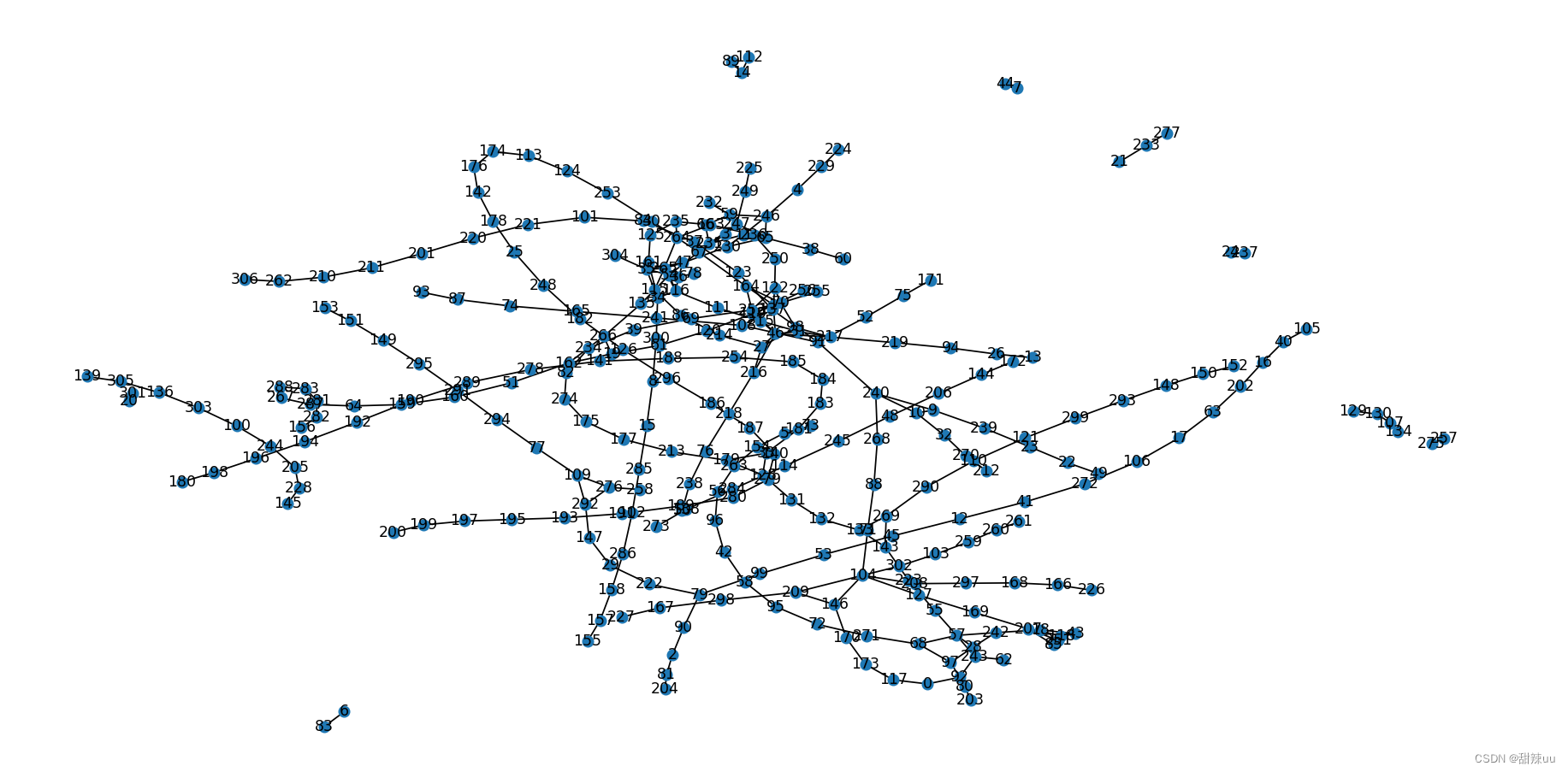
data=pd.read_csv('datasets/graph.csv')
data=data.values
print(data.shape)

import numpy as np
from scipy.sparse import csr_matrix


# 假设有5个节点，节点对应关系如下（示例数据）
node_relations=[]
for line in data:
    my_tuple = (int(line[0]),int(line[1]))
    node_relations.append(my_tuple)

# 计算节点的个数
num_nodes = max(max(edge) for edge in node_relations) + 1

# 构建初始邻接矩阵
adj_matrix = np.zeros((num_nodes, num_nodes))

# 填充邻接矩阵
for edge in node_relations:
    adj_matrix[edge[0], edge[1]] = 1
    adj_matrix[edge[1], edge[0]] = 1  # 如果是无向图，需对称填充

# 将邻接矩阵转换为稀疏矩阵（这里使用 CSR 稀疏格式）
sparse_adj_matrix = csr_matrix(adj_matrix)

print("邻接矩阵：")
print(adj_matrix.shape)
# print("\n稀疏矩阵表示：")
# print(sparse_adj_matrix.shape)
A = torch.Tensor(adj_matrix)# torch.rand((num_nodes, num_nodes))  # 邻接矩阵
print(A.shape)
X = torch.rand((num_nodes, 64))  # 特征矩阵，假设每个节点有10维特征
print(X.shape)

# 定义图卷积层
class GraphConvLayer(nn.Module):
    def __init__(self, in_features, out_features):
        super(GraphConvLayer, self).__init__()
        self.linear = nn.Linear(in_features, out_features)

    def forward(self, A, X):
        AX = torch.matmul(A, X)  # 对特征矩阵和邻接矩阵进行乘积操作
        return self.linear(AX)  # 返回线性层的输出


# 定义简单的GCN模型
class SimpleGCN(nn.Module):
    def __init__(self, in_features, hidden_features, out_features):
        super(SimpleGCN, self).__init__()
        self.conv1 = GraphConvLayer(in_features, hidden_features)
        self.conv2 = GraphConvLayer(hidden_features, out_features)

    def forward(self, A, X):
        h = torch.relu(self.conv1(A, X))  # 第一个图卷积层
        out = self.conv2(A, h)  # 第二个图卷积层
        return out


# 初始化GCN模型
gcn_model = SimpleGCN(in_features=64, hidden_features=128, out_features=64)  # 输入特征为10维，隐藏层特征为16维，输出为8维

# 损失函数和优化器
criterion = nn.MSELoss()  # 均方误差损失函数
optimizer = optim.Adam(gcn_model.parameters(), lr=0.01)  # Adam优化器

# 训练模型
num_epochs = 1000
for epoch in range(num_epochs):
    optimizer.zero_grad()
    output = gcn_model(A, X)
    loss = criterion(output, torch.zeros_like(output))  # 示范用零向量作为目标值，实际情况需要根据具体任务调整
    loss.backward()
    optimizer.step()

    if (epoch + 1) % 100 == 0:
        print(f'Epoch [{epoch + 1}/{num_epochs}], Loss: {loss.item()}')

# 得到节点的向量化表示
node_embeddings = gcn_model(A, X)
print("节点的向量化表示：")
print(node_embeddings.shape)