本文仅供学习使用
本文参考:
B站:DR_CAN
Dr. CAN学习笔记 - Ch02动态系统建模与分析
- 1. 课程介绍
- 2. 电路系统建模、基尔霍夫定律
- 3. 流体系统建模
- 4. 拉普拉斯变换(Laplace)传递函数、微分方程
- 4.1 Laplace Transform 拉式变换
- 4.2 收敛域(ROC)与逆变换(ILT)
- 4.3 传递函数 Transfer Function
- 5. 一阶系统的单位阶跃响应(step response),时间常数(Time Constant)
- 6. 频率响应与滤波器
- 7. 二阶系统
- 7.1 二阶系统对初始条件的动态响应 Matlab/Simulink - 2nd Order Syetem Response to IC
- 7.2 二阶系统的单位阶跃响应 2nd Order System Unit Step Response
- 7.3 二阶系统单位阶跃的性能分析与比较 2nd Order System Unit Step Response
- 7.4 共振现象-二阶系统频率响应,现象部分
- 7.5 二阶系统的频率响应
- 8. 二阶系统的频率响应
1. 课程介绍

2. 电路系统建模、基尔霍夫定律
基本元件:
电量 库伦(
C
C
C)
q
q
q
电流 安培(
A
A
A)
i
i
i ——
i
=
d
e
d
t
i=\frac{\mathrm{d}e}{\mathrm{d}t}
i=dtde 流速
电压 伏特(
V
V
V)
e
e
e
电阻 欧姆(
Ω
\varOmega
Ω)
R
R
R ——
e
R
=
i
R
e_{\mathrm{R}}=iR
eR=iR
电容 法拉(
F
F
F)
C
C
C ——
q
=
C
e
C
,
e
C
=
1
C
q
=
1
C
∫
0
t
i
d
t
q=Ce_{\mathrm{C}},e_{\mathrm{C}}=\frac{1}{C}q=\frac{1}{C}\int_0^t{i}\mathrm{d}t
q=CeC,eC=C1q=C1∫0tidt
电感 亨利(
H
H
H)
L
L
L ——
e
L
=
L
d
i
d
t
=
L
i
′
e_{\mathrm{L}}=L\frac{\mathrm{d}i}{\mathrm{d}t}=Li^{\prime}
eL=Ldtdi=Li′

基尔霍夫定律
K(Kirchhoff) C(Current) L(Law) —— 所有进入某节点的电流的总和等于所有离开这个节点的的电流总和
K(Kirchhoff) V(Voltage) L(Law) —— 沿着闭合回路所有元件两端的电压的代数和等于零

 )
)
3. 流体系统建模

流量 flow rate
q
q
q
m
3
/
s
m^3/s
m3/s
体积 volume
V
V
V
m
3
m^3
m3
高度 heigh
h
h
h
m
m
m
压强 pressure
p
p
p
N
/
m
(
p
a
s
c
a
l
)
N/m\left( pascal \right)
N/m(pascal)
静压 Hydrostatic Pressure
p
H
y
d
r
o
=
F
H
y
d
r
o
A
=
m
g
A
=
ρ
g
h
p_{\mathrm{Hydro}}=\frac{F_{\mathrm{Hydro}}}{A}=\frac{mg}{A}=\rho gh
pHydro=AFHydro=Amg=ρgh
绝对压强 Asolute Pressure
p
a
b
s
=
p
a
+
p
H
y
d
r
o
=
p
a
+
ρ
g
h
p_{abs}=p_{\mathrm{a}}+p_{\mathrm{Hydro}}=p_{\mathrm{a}}+\rho gh
pabs=pa+pHydro=pa+ρgh
表压 Gauge Pressure
P
g
a
u
g
e
=
p
a
b
s
−
p
a
=
ρ
g
h
P_{\mathrm{gauge}}=p_{abs}-p_{\mathrm{a}}=\rho gh
Pgauge=pabs−pa=ρgh
流阻 Fluid Resistance

质量守恒 Conservation of Mass

4. 拉普拉斯变换(Laplace)传递函数、微分方程
4.1 Laplace Transform 拉式变换
f
(
t
)
→
F
(
s
)
f\left( t \right) \rightarrow F\left( s \right)
f(t)→F(s) : 时域 - 频域
s
=
σ
+
j
w
s=\sigma +jw
s=σ+jw


4.2 收敛域(ROC)与逆变换(ILT)


微分方程——描述动态世界
状态变量 :
d
x
⃗
d
t
\frac{\mathrm{d}\vec{x}}{\mathrm{d}t}
dtdx-时间
位移:
s
s
s , 速度:
d
x
d
t
\frac{\mathrm{d}x}{\mathrm{d}t}
dtdx ,加速度:
d
2
x
d
t
2
\frac{\mathrm{d}^2x}{\mathrm{d}t^2}
dt2d2x
- F = m d 2 x d t 2 F=m\frac{\mathrm{d}^2x}{\mathrm{d}t^2} F=mdt2d2x
- d T d t = − k ( T − C ) \frac{\mathrm{d}T}{\mathrm{d}t}=-k\left( T-C \right) dtdT=−k(T−C)
- d P d t = − r p ( 1 − p k ) \frac{\mathrm{d}P}{\mathrm{d}t}=-rp\left( 1-\frac{p}{k} \right) dtdP=−rp(1−kp) 人口增长
常系数线性 —— 线性时不变系统
- 求解 3Step
从 t t t— s s s L [ f ( t ) ] \mathcal{L} \left[ f\left( t \right) \right] L[f(t)]
运算求解
从 s s s— t t t L − 1 [ F ( s ) ] \mathcal{L} ^{-1}\left[ F\left( s \right) \right] L−1[F(s)]
非线性
- 线性化
- 非线性分析控制

4.3 传递函数 Transfer Function
——根轨迹 BodePlot 信号处理


5. 一阶系统的单位阶跃响应(step response),时间常数(Time Constant)

换个角度分析单位阶跃响应(System Unit Step Response - 一阶 1st order)——LTI
一阶线性时不变 —— 1st order LTI
x
˙
+
a
x
=
a
u
x
(
0
)
=
x
˙
(
0
)
=
0
\dot{x}+ax=au \\ x\left( 0 \right) =\dot{x}\left( 0 \right) =0
x˙+ax=aux(0)=x˙(0)=0
传递函数 : s X ( s ) + a X ( s ) = a U ( s ) ; H ( s ) = X ( s ) U ( s ) = a s + a sX\left( s \right) +aX\left( s \right) =aU\left( s \right) ;H\left( s \right) =\frac{X\left( s \right)}{U\left( s \right)}=\frac{a}{s+a} sX(s)+aX(s)=aU(s);H(s)=U(s)X(s)=s+aa

Another Viewpoint :
x
˙
+
a
x
=
a
u
,
t
⩾
0
,
u
=
1
⇒
x
˙
=
a
−
a
x
=
a
(
1
−
x
)
\dot{x}+ax=au,t\geqslant 0,u=1\Rightarrow \dot{x}=a-ax=a\left( 1-x \right)
x˙+ax=au,t⩾0,u=1⇒x˙=a−ax=a(1−x)

6. 频率响应与滤波器


1st order system 一阶系统

低通滤波器——Loss Pass Filter

7. 二阶系统
7.1 二阶系统对初始条件的动态响应 Matlab/Simulink - 2nd Order Syetem Response to IC
Vibration 振动


7.2 二阶系统的单位阶跃响应 2nd Order System Unit Step Response

Unit Step Imput 单位阶跃


7.3 二阶系统单位阶跃的性能分析与比较 2nd Order System Unit Step Response


7.4 共振现象-二阶系统频率响应,现象部分

7.5 二阶系统的频率响应

8. 二阶系统的频率响应

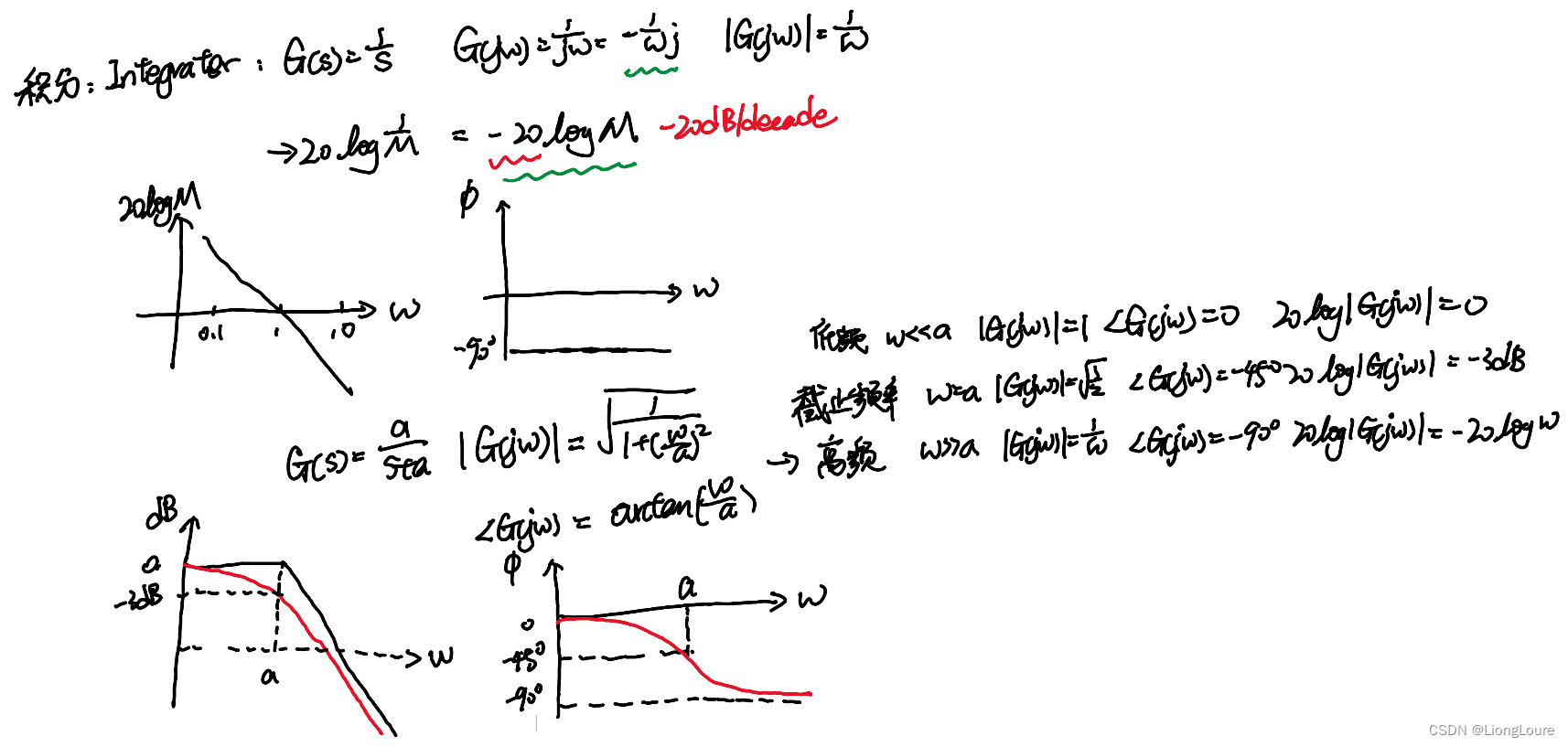
Bode Plot 手绘技巧与应用