本文将讲解,PyTorch卷积神经网络各层实现与介绍,包括:基本骨架–nn.Module的使用、卷积操作、卷积层、池化层、激活函数、全连接层的介绍。
😜 对于相关原理,可以跳转👉卷积神经网络CNN各层基本知识
😜 后续会以CIFAR10数据集作为案例,关于CIFAR10数据集在上篇中有详细的介绍,可以跳转👉Pytorch公共数据集、tensorboard、DataLoader使用。
基本骨架–nn.Module的使用
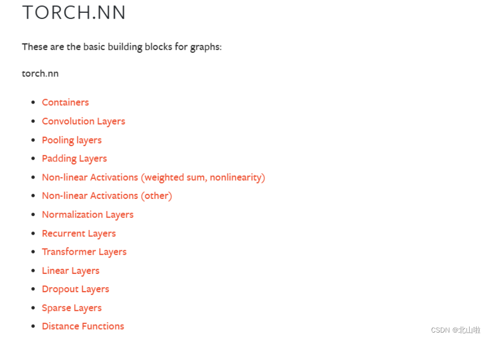
torch.nn模块包含着torch已经准备好的层,方便使用者调用构建网络,一下内容包括nnModule而极少、卷积操作的简单操作、卷积层、池化层、激活函数、全连接层以及其他层的相关使用方法
neural network
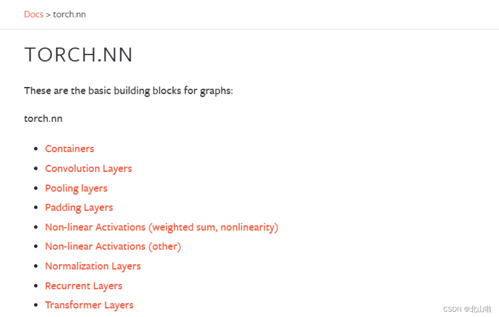
torch.nn模块包含着torch已经准备好的层,方便使用者调用构建网络。后文将介绍卷积层、池化层、激活函数层、循环层、全连接层的相关使用方法。
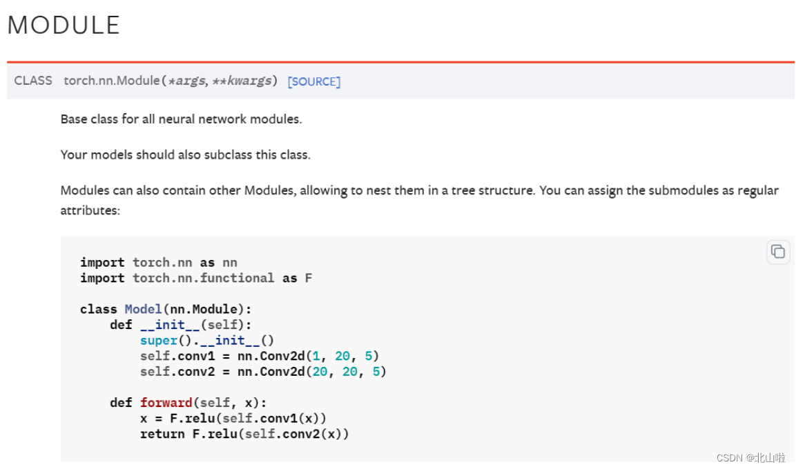
Module:位于containers容器中
'''神经网络模板'''
#https://beishan.blog.csdn.net/
import torch.nn as nn
import torch.nn.functional as F


class Model(nn.Module):  # nn.Module为其父类,Model继承它

    def __init__(self):
        super().__init__()  #调用父类的初始化函数
        self.conv1 = nn.Conv2d(1, 20, 5)
        self.conv2 = nn.Conv2d(20, 20, 5)

    def forward(self, x):  #用于定义神经网络的前向传播过程
        x = F.relu(self.conv1(x))  #卷积->非线性处理
        return F.relu(self.conv2(x))  #卷积->非线性处理->return
代码解释如下:
forward 函数是深度学习框架中常见的一个函数,用于定义神经网络的前向传播过程。
forward 函数的作用是将输入数据经过网络中各个层的计算和变换后,得到输出结果。
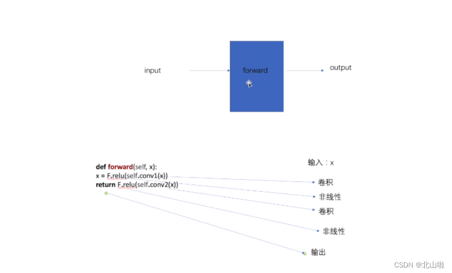
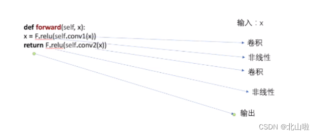
在上述代码中,forward函数:对输入的x进行第一次卷积,再进行第一次非线性操作;再第二次进行卷积,然后第二次非线性操作。最后返回结果。
搭建自己的网络
import torch.nn as nn
import torch
class Beishan(nn.Module):

    def __init__(self):
        super().__init__()

    def forward(self, input):
        output = input * 2
        return output


bs = Beishan()
x = torch.tensor(1.0)
print(bs(x))
tensor(2.)
卷积操作
卷积可以看作输入和卷积核之间的内积运算,是两个实值函数之间的一种数学运算
在Pytorch中针对卷积操作的对象和使用场景的不同,有一维卷积、二维卷积、三位卷积与转置卷积(可以简单理解为卷积操作的逆操作),但他们的使用方法类似,都可以从torch.nn模块中调用
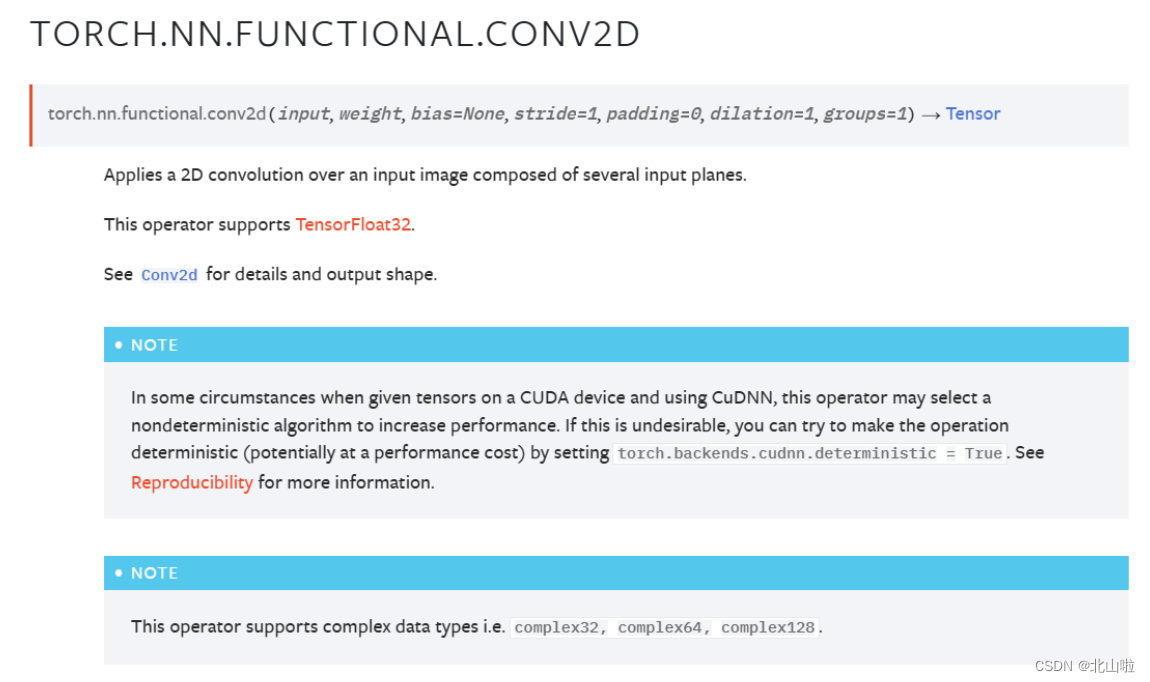
接下来将以torch.nn.functional.conv2d()为例进行讲解,后续的层的讲解,将以torch.nn作为案例
torch.nn.functional.conv2d(input,
                           weight,
                           bias=None,
                           stride=1,
                           padding=0,
                           dilation=1,
                           groups=1)
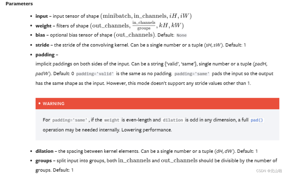
| 参数 | 解释 |
|---|---|
| input | 输入图像的通道数 |
| weight | 卷积核的大小 |
| bias | 可选的偏置张量的形状(输出通道)(输出通道),默认值:无 |
| stride | 卷积的步长,默认为1 |
| padding | 在输入两边进行0填充的数量,默认为0 |
| dilation | 控制卷积核之间的间距 |
需要注意的是: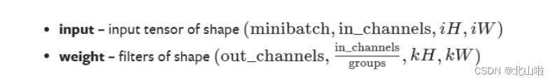
input中的shape:
- minibatch:batch中的样例个数,
- in_channels:每个样例数据的通道数,
- iH:每个样例的高(行数),
- iW:每个样例的宽(列数)
weight中的shape:
- out_channels:卷积核的个数
- in_channels/groups:每个卷积核的通道数
- kH:每个卷积核的高(行数)
- kW:每个卷积核的宽(列数)
- padding
就是填充的意思,将图像数据的边缘部分填充的大小,通过padding可以使得卷积过程中提取到图像边缘部分的信息 - stride
卷积核移动的步长,即卷积核完成局部的一次卷积后向右移动的步数,步长增大可以减小特征图的尺寸计算速度提升。适用于高分辨率的图像
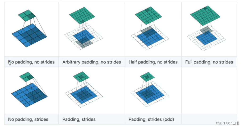
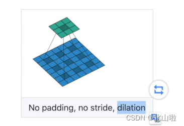
接下来将以下图的卷积操作,其中padding和stride都是默认值。即padding=0,stride=1,利用Pytorch进行验证运算
import torch.nn.functional as F
import torch

# input
input_ = torch.tensor([[3, 3, 2, 1, 0],
                       [0, 0, 1, 3, 1],
                       [3, 1, 2, 2, 3],
                       [2, 0, 0, 2, 2],
                       [2, 0, 0, 0, 1]])
# 卷积核
kernel = torch.tensor([[0, 1, 2],
                       [2, 2, 0],
                       [0, 1, 2]])

# print,input_.shape,kernel.shape
print(input_.shape)
print(kernel.shape)
# 由上面可以知道.shape不满足需求,而是只有h和w的2个数据,利用reshape进行变换

input_ = torch.reshape(input_, (1, 1, 5, 5))  # 表示样例个数1,每一个样例数据的通道数1,高5,宽5
kernel = torch.reshape(kernel, (1, 1, 3, 3))

# 进行conv2d卷积运算
output = F.conv2d(input_, kernel, stride=1)  # stride=1即每一次只进行一步移动操作
print(output)
torch.Size([5, 5])
torch.Size([3, 3])
tensor([[[[12, 12, 17],
          [10, 17, 19],
          [ 9,  6, 14]]]])
在后续的层的讲解中,将以torch.nn作为案例。后续会更新
卷积层
这里主要介绍代码部分,对于相关原理,可以查看 https://beishan.blog.csdn.net/article/details/128058839
import torch.nn as nn
#其中in_channels,ut_channels,kernel_size需要进行设置,其他均有默认值
torch.nn.Conv2d(in_channels,
                out_channels,
                kernel_size,
                stride=1,
                padding=0,
                dilation=1,
                groups=1,
                bias=True,
                padding_mode='zeros',
                device=None,
                dtype=None)
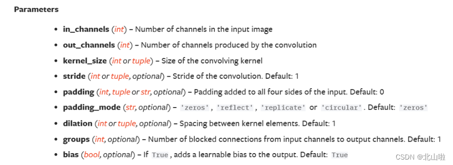
常用的参数为:in_channels 、out_channels 、kernel_size 、stride 、padding
| Conv2d参数 | 说明 |
|---|---|
| in_channels | 表示输入的图片通道数目。 |
| out_channels | 表示输出的图片通道数目。 |
| kernel_size | 表示卷积核的大小,当卷积是正方形的时候,只需要一个整数边长即可,卷积不是正方形,要输入一个元组表示高和宽。 |
| stride | 表示每次卷积核移动的步长值。 |
| padding | 表示是否添加边界,一旦设置就是四周都添加。在原始的行列基础上,行增加2行,列增加2列。 |
| dilation | 表示控制卷积核之间的间距。 |
| groups | 表示控制输入和输出之间的连接。 |
| bias | 表示是否将一个 bias 增加到输出。 |
| padding_mode | 表示接收’zeros’, ‘reflect’, ‘replicate’ or ‘circular’. Default: ‘zeros’,默认是’zeros’,即默认在padding操作时,在外一圈是填充的0。 |
卷积层操作实战
下面代码以CIFAR10数据集为例进行实践
关于CIFAR10数据集在上篇中有详细的介绍,可以跳转☞Pytorch公共数据集、tensorboard、DataLoader使用。后续的操作也是以CIFAR10数据集为案例
import torch
import torchvision
import torch.nn as nn
from torch.utils.data import DataLoader
dataset = torchvision.datasets.CIFAR10("dataset",train=False,transform=torchvision.transforms.ToTensor(),download=True)
dataloader = DataLoader(dataset,batch_size=64)
Files already downloaded and verified
class BS(torch.nn.Module):
    def __init__(self):
        super().__init__()
        # 即输入通道设定为RGB3层,输出通道设定为6,卷积核大小为3,步长设定1,不进行填充
        self.conv1 = nn.Conv2d(in_channels=3,
                               out_channels=6,
                               kernel_size=3,
                               stride=1,
                               padding=0)

    def forward(self,x):
        return self.conv2(x)
bs = BS()
print(bs)  # 打印创建的卷积参数
BS(
  (conv1): Conv2d(3, 6, kernel_size=(3, 3), stride=(1, 1))
)
#input:torch.Size([64, 3, 32, 32])
#output:torch.Size([64, 6, 32, 32])
从输出结果可知,输入通道为3,输出通道为6,卷积核结构为3×3,步长为1
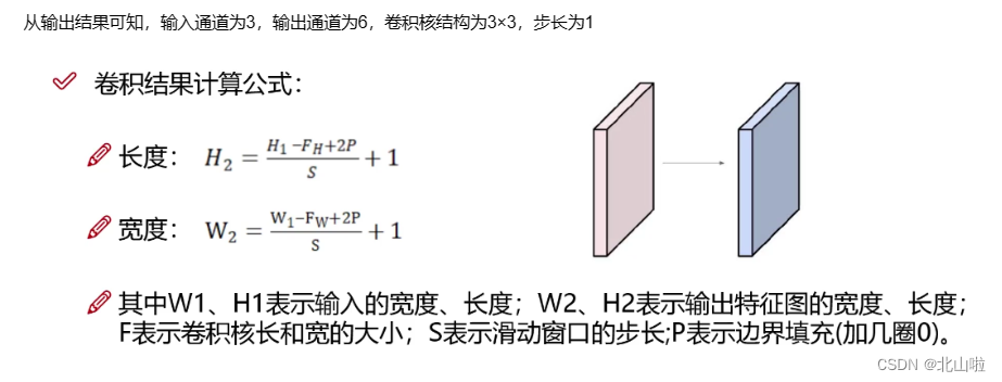
按计算可得,输出特征图的尺寸:
( 32 − 3 + 2 ∗ 0 ) 1 (32 - 3 + 2*0)\over1 1(32−3+2∗0) + 1 = 30
完整代码如下:
import torch
import torchvision
from torch.utils.data import DataLoader
from torch.utils.tensorboard import SummaryWriter
dataset = torchvision.datasets.CIFAR10(
"dataset",
train=False,
transform=torchvision.transforms.ToTensor(),
download=True)
# 加载数据集,每次从数据集中取64
dataloader = DataLoader(dataset, batch_size=64)
class BS(torch.nn.Module):
def __init__(self):
super().__init__()
# 即输入通道设定为RGB3层,输出通道设定为6,卷积核大小为3,步长设定1,不进行填充
self.conv2 = torch.nn.Conv2d(in_channels=3,
out_channels=6,
kernel_size=3,
stride=1,
padding=0)
def forward(self, x):
return self.conv2(x)
step = 0
writer = SummaryWriter('logs')
for data in dataloader:
img, target = data
# 卷积前
print(img.shape)
# 卷积后
output = BS().conv2(img)
#print(output.shape)
#input:torch.Size([64, 3, 32, 32])
#output:torch.Size([64, 6, 32, 32])
output=output.reshape(-1,3,30,30) #output的channel为6,此时在Tensorboard可视化中无法显示通道为6的图片,所以需要进行reshape进行重新设定。
print(output.shape)
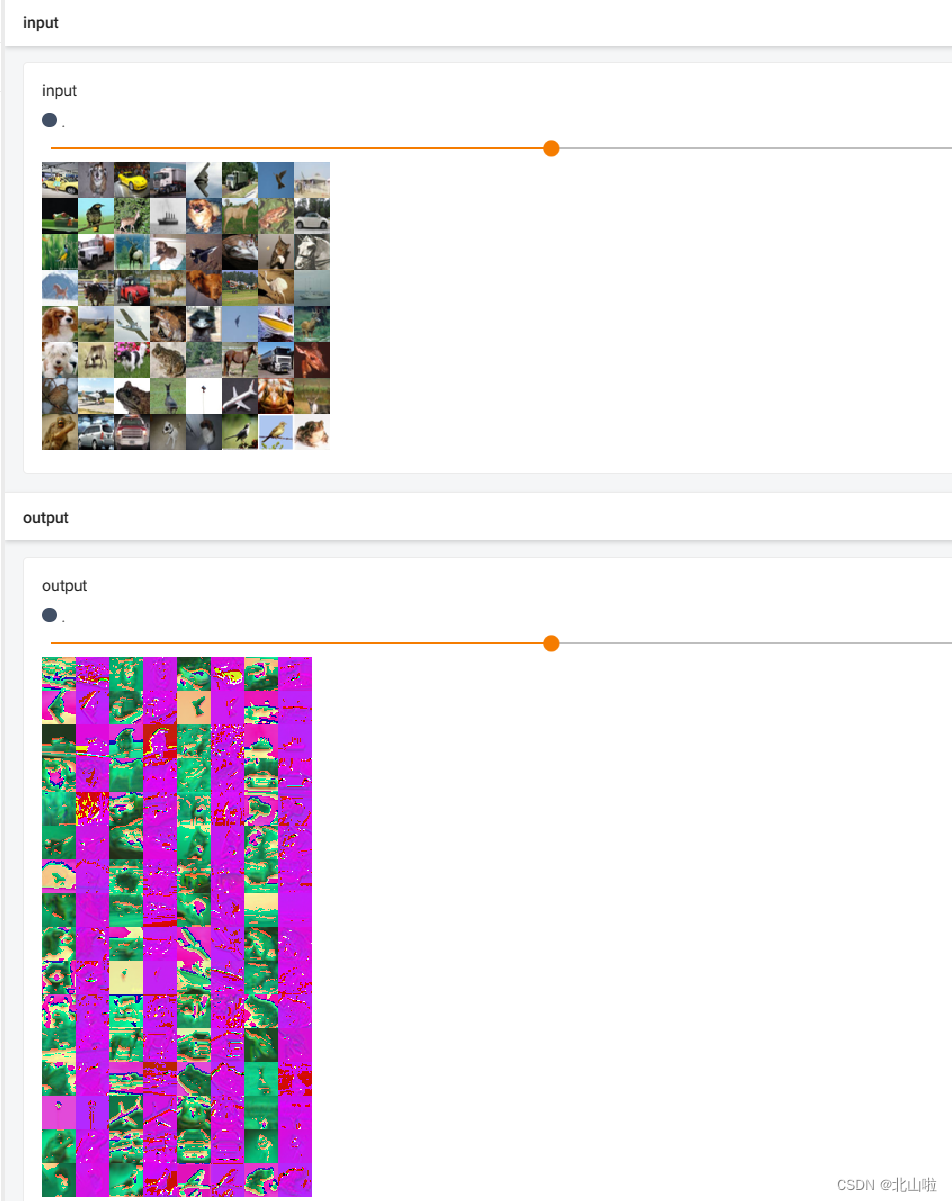
writer.add_images('input',img,step)
writer.add_images('output',output,step)
step += 1
writer.close()
Files already downloaded and verified
torch.Size([64, 3, 32, 32])
torch.Size([128, 3, 30, 30])
torch.Size([64, 3, 32, 32])
torch.Size([128, 3, 30, 30])
.......
tensorboard显示如下
池化层
池化操作主要用于减小特征图的尺寸,并提取出最重要的特征
它通过在特定区域内进行汇总或聚合来实现这一目标。
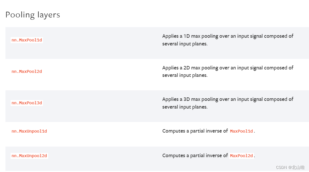
池化层的常见操作包含以下几种:最大值池化,均值池化,随机池化,中值池化,组合池化等。后续以torch.nn.MaxPool2d为例,进行介绍
torch.nn.MaxPool2d(kernel_size,
                   stride=None,
                   padding=0,
                   dilation=1,
                   return_indices=False,
                   ceil_mode=False)
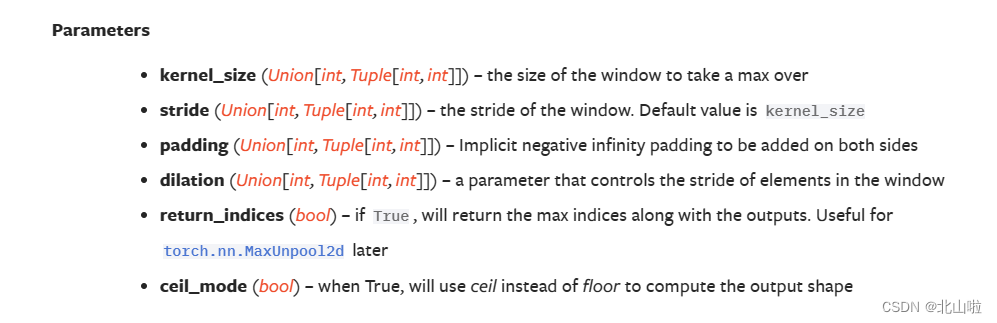

其他参数与池化层中相似,有些默认参数不同而已,这次讲解dilation、ceil_mode
dilation:表示设置核的膨胀率,默认 dilation=1,即如果kernel_size =3,那么核的大小就是3×3。如果dilation = 2,kernel_size =3×3,那么每列数据与每列数据,每行数据与每行数据中间都再加一行或列数据,数据都用0填充,那么核的大小就变成5×5。
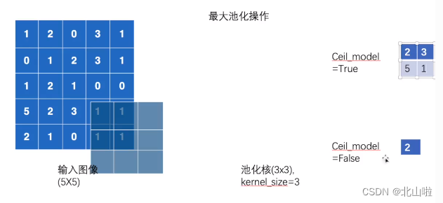
ceil_mode:floor or ceiling,表示计算输出结果形状的时候,是使用向上取整还是向下取整。即要不要舍弃无法覆盖核的大小的数值。True为保留,False为舍弃
下图为max_pooling的动态演示图
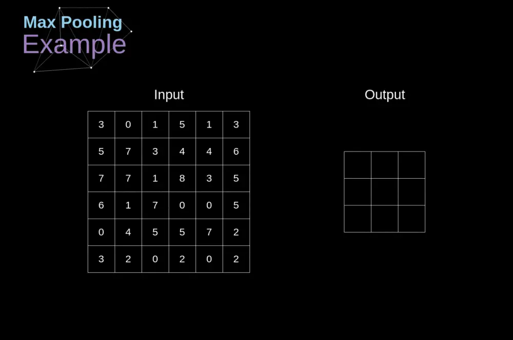
利用pytorch演算结果
import torch
from torch import nn

input = torch.tensor(
    [[3, 0, 1, 5, 1, 3], [5, 7, 3, 4, 4, 6], [7, 7, 1, 8, 3, 5],
     [6, 1, 7, 0, 0, 5], [0, 4, 5, 5, 7, 2], [3, 2, 0, 2, 0, 2]],
    dtype=float)  # 使用dtype将此矩阵的数字变为浮点型
# 准备的参数情况
print(input.shape)
# 进行reshape
input = torch.reshape(input, (1,1,6,6))  # input:(N,C,H,W)or(C,H,W)
print(input.shape)


# 搭建神经网络并进行池化操作
class BS(nn.Module):

    def __init__(self):
        super().__init__()
        self.maxpool2 = nn.MaxPool2d(kernel_size=2, ceil_mode=True)

    def forward(self, input):
        output = self.maxpool2(input)
        return output


# 实例化
bs = BS()
output = bs(input)
print(output)
torch.Size([6, 6])
torch.Size([1, 1, 6, 6])
tensor([[[[7., 5., 6.],
          [7., 8., 5.],
          [4., 5., 7.]]]], dtype=torch.float64)
利用最大池化处理CIFAR10数据集图片,并利用tensorboard可视化
#https://beishan.blog.csdn.net/
import torch
import torch.nn as nn
import torchvision
from torch.utils.data import DataLoader
from torch.utils.tensorboard import SummaryWriter
dataset = torchvision.datasets.CIFAR10(
    "dataset",
    train=False,
    transform=torchvision.transforms.ToTensor(),
    download=True)
# 加载数据集,每次从数据集中取64
dataloader = DataLoader(dataset, batch_size=64)


class BS(nn.Module):

    def __init__(self):
        super().__init__()
        self.maxpool1 = nn.MaxPool2d(kernel_size=2, ceil_mode=True)

    def forward(self, input):
        output = self.maxpool1(input)
        return output


step = 0
bs = BS()
writer = SummaryWriter('logs')
for data in dataloader:
    img, target = data
    output = bs(img)
    writer.add_images('input_maxpool', img, step)
    writer.add_images('output_maxpool', output, step)
    step += 1
writer.close()
Files already downloaded and verified
tensorboard显示如下

非线性激活
激活函数的作用在于提供网络的非线性建模能力,如果不用激励函数,每一层输出都是上层输入的线性函数,无论神经网络有多少层,输出都是输入的线性组合,这种情况就是最原始的感知机。
激活函数给神经元引入了非线性因素,使得神经网络可以任意逼近任何非线性函数,这样神经网络就可以应用到众多的非线性模型中。
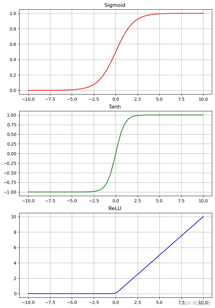
常见的包括:sigmoid、relu和tanh,后续将以relu进行介绍
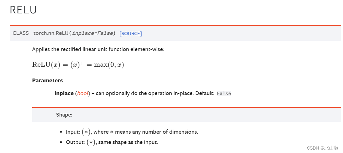
使用relu处理矩阵
import torch

# 准备数据
input = torch.tensor([[1, -1, 0], [-2, 3, -6]])


# 搭建自己的一个神经网络
class BS(torch.nn.Module):

    def __init__(self):
        super().__init__()
        # 默认inplace参数为False
        self.relu1 = torch.nn.ReLU(inplace=False) #inplace保留原始数据

    def forward(self, input):
        output = self.relu1(input)
        return output


# 实例化
l = BS()
output = l(input)
print('转换前:', input)
print('relu转换后:', output)
转换前: tensor([[ 1, -1,  0],
        [-2,  3, -6]])
relu转换后: tensor([[1, 0, 0],
        [0, 3, 0]])
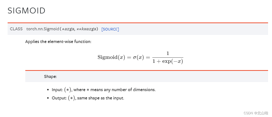
利用Sigmoid来处理CIFAR10数据集
import torch
import torch.nn as nn
import torchvision
from torch.utils.data import DataLoader
from torch.utils.tensorboard import SummaryWriter
dataset = torchvision.datasets.CIFAR10(
    "dataset",
    train=False,
    transform=torchvision.transforms.ToTensor(),
    download=True)
# 加载数据集,每次从数据集中取64
dataloader = DataLoader(dataset, batch_size=64)


class BS(nn.Module):

    def __init__(self):
        super().__init__()
        self.sigmoid1 = nn.Sigmoid()

    def forward(self, input):
        output = self.sigmoid1(input)
        return output


step = 0
bs = BS()
writer = SummaryWriter('logs')
for data in dataloader:
    img, target = data
    output = bs(img)
    writer.add_images('input_sigmoid', img, step)
    writer.add_images('output_sigmoid', output, step)
    step += 1
writer.close()
Files already downloaded and verified
tensorboard显示如下

全连接层
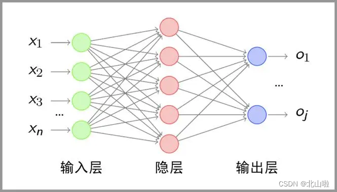
线性层它也被称为全连接层,通常所说的全连接层是指一个由多个神经元所组成的层,其所有的输出和该层的所有输入都有连接,即每个输入都会影响所有神经元的输出,在Pytorch中nn.Linear()表示线性变换
全连接层可以看作是nn.Linear()表示线性层再加上一个激活函数所构成的结构。
全连接层的应用范围非常广泛,只有全连接层组成的网络是全连接神经网络,可以用于数据的分类或回归任务,卷积神经网络和循环神经网络的末端通常会由多个全连接层组成
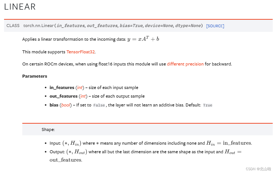
torch.nn.Linear(in_features,
				out_features,
				bias=True,
 			    device=None,
				dtype=None)
其中最重要的三个参数为in_features, out_features, bias
- in_features:表示输入的特征值大小,即输入的神经元个数
- out_features:表示输出的特征值大小,即经过线性变换后输出的神经元个数
- bias:表示是否添加偏置
以VGG16网络结构为例进行介绍
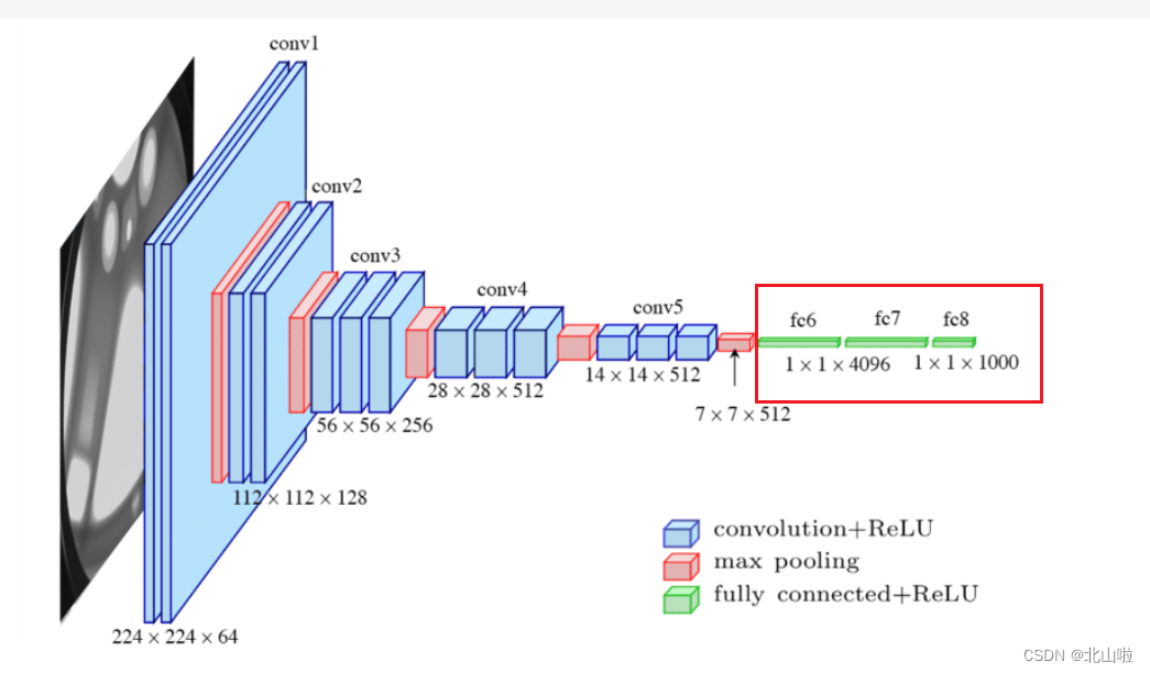
in_features为1,1,x形式,out_features为1,1,y的形式
import torch
import torchvision
from torch.utils.data import DataLoader

# 准备数据
test_set = torchvision.datasets.CIFAR10("dataset",
                                        train=False,
                                        transform=torchvision.transforms.ToTensor(),
                                        download=True)
# 加载数据集
dataloader = DataLoader(test_set,batch_size=64)

# 查看输入的通道数
# for data in dataloader:
#     imgs, target = data
#     print(imgs.shape)  # torch.Size([64, 3, 32, 32])
#     # 将img进行reshape成1,1,x的形式
#     input = torch.reshape(imgs,(1,1,1,-1)) # 每次一张图,1通道,1*自动计算x
#     print(input.shape) # torch.Size([1, 1, 1, 196608])

# 搭建神经网络,设置预定的输出特征值为10
class BS(torch.nn.Module):
    def __init__(self):
        super().__init__()
        self.linear1 = torch.nn.Linear(196608,10)  # 输入数据的特征值196608,输出特征值10
    def forward(self, input):
        output = self.linear1(input)
        return output

l = BS()
for data in dataloader:
    imgs, target = data
    print(f"原先的图片shape:{imgs.shape}")  # torch.Size([64, 3, 32, 32])
    # 将img进行reshape成1,1,x的形式
    input = torch.flatten(imgs) # 每次一张图,1通道,1*自动计算x
    print(f"flatten后的图片shape:{input.shape}")
    output = l(input)
    print(f"经过线性后的图片shape:{output.shape}") # torch.Size([1, 1, 1, 10])
Files already downloaded and verified
原先的图片shape:torch.Size([64, 3, 32, 32])
flatten后的图片shape:torch.Size([196608])
经过线性后的图片shape:torch.Size([10])
原先的图片shape:torch.Size([64, 3, 32, 32])
flatten后的图片shape:torch.Size([19660
关于神经网络的层结构远不止这些,例如dropout layers、transformer layers、recurrent layers等,大家可以去官网自行学习