【Sklearn】基于最中心分类器算法的数据分类预测(Excel可直接替换数据)
- 1.模型原理
- 2.模型参数
- 3.文件结构
- 4.Excel数据
- 5.下载地址
- 6.完整代码
- 7.运行结果
1.模型原理
最近中心分类器(Nearest Centroid Classifier)也被称为近似最近邻分类器(Nearest Shrunken Centroid Classifier)。它是一种基于类别中心的分类方法,适用于线性可分问题。其基本思想是将每个类别的样本特征取平均,得到每个类别的中心点,然后将待分类样本与这些中心点进行距离比较,将其分配给距离最近的类别。
以下是最近中心分类器的模型原理及数学公式:
模型原理:
- 对于每个类别,计算其样本特征的平均值,得到类别的中心点。
- 对于一个待分类的样本,计算其与每个类别中心点的距离,然后将其分配给距离最近的类别。
数学模型:
- 对于类别 c c c,其样本特征的平均值为 μ c = 1 N c ∑ i = 1 N c x i c \mu_c = \frac{1}{N_c} \sum_{i=1}^{N_c} x_i^c μc=Nc1∑i=1Ncxic,其中 N c N_c Nc 是属于类别 c c c 的样本数量, x i c x_i^c xic 是类别 c c c 中的第 i i i 个样本的特征。
- 对于一个待分类的样本 x x x,将其分配给距离最近的中心点,即 y = arg min c ∥ x − μ c ∥ 2 2 y = \arg \min_{c} \|x - \mu_c\|_2^2 y=argminc∥x−μc∥22,其中 ∥ x − μ c ∥ 2 2 \|x - \mu_c\|_2^2 ∥x−μc∥22 表示欧氏距离的平方。
此外,为了减少特征的影响,最近中心分类器还可以引入一个收缩参数,将各个特征的权重进行缩减,从而更关注对分类有用的特征。
虽然最近中心分类器简单,但在某些情况下,它可以表现得非常好。然而,它的性能在数据分布不均衡或特征相关性较大时可能下降。在实际应用中,您可以根据数据集的特点选择最适合的分类方法。
2.模型参数
NearestCentroid类在Scikit-Learn中没有太多的参数可以调整,它主要用于简单的最近中心分类任务。以下是该类的参数列表和一个简单的示例:
参数列表:
metric: 指定用于计算距离的距离度量,默认为欧氏距离。可选值包括:“euclidean”、“manhattan”、"cosine"等。
3.文件结构

iris.xlsx						% 可替换数据集
Main.py							% 主函数
4.Excel数据

5.下载地址
- 资源下载地址
6.完整代码
import pandas as pd
from sklearn.model_selection import train_test_split
from sklearn.neighbors import NearestCentroid
from sklearn.metrics import accuracy_score, confusion_matrix
import matplotlib.pyplot as plt
import seaborn as sns

def nearest_centroid_classification(data_path, test_size=0.2, random_state=42):
    # 加载数据
    data = pd.read_excel(data_path)

    # 分割特征和标签
    X = data.iloc[:, :-1]  # 所有列除了最后一列
    y = data.iloc[:, -1]   # 最后一列

    # 划分训练集和测试集
    X_train, X_test, y_train, y_test = train_test_split(X, y, test_size=test_size, random_state=random_state)

    # 创建最近中心分类器模型
    # ** 参数列表 **:
    # `metric`: 指定用于计算距离的距离度量,默认为欧氏距离。可选值包括:"euclidean"、"manhattan"、"cosine"等。
    model = NearestCentroid(metric="manhattan")

    # 在训练集上训练模型
    model.fit(X_train, y_train)

    # 在测试集上进行预测
    y_pred = model.predict(X_test)

    # 计算准确率
    accuracy = accuracy_score(y_test, y_pred)
    return confusion_matrix(y_test, y_pred), y_test.values, y_pred, accuracy

if __name__ == "__main__":
    # 使用函数进行分类任务
    data_path = "iris.xlsx"
    confusion_mat, true_labels, predicted_labels, accuracy = nearest_centroid_classification(data_path)

    print("真实值:", true_labels)
    print("预测值:", predicted_labels)
    print("准确率:{:.2%}".format(accuracy))

    # 绘制混淆矩阵
    plt.figure(figsize=(8, 6))
    sns.heatmap(confusion_mat, annot=True, fmt="d", cmap="Blues")
    plt.title("Confusion Matrix")
    plt.xlabel("Predicted Labels")
    plt.ylabel("True Labels")
    plt.show()

    # 用圆圈表示真实值,用叉叉表示预测值
    # 绘制真实值与预测值的对比结果
    plt.figure(figsize=(10, 6))
    plt.plot(true_labels, 'o', label="True Labels")
    plt.plot(predicted_labels, 'x', label="Predicted Labels")

    plt.title("True Labels vs Predicted Labels")
    plt.xlabel("Sample Index")
    plt.ylabel("Label")
    plt.legend()
    plt.show()
7.运行结果