在前面的博文:
《参数量仅有50KB的超轻量级unet变种网络egeunet【参数和计算量降低494和160倍】医疗图像分割实践》
初步学习和实践了最新的超轻量级的unet变种网络在医疗图像领域内的表现,在上文中我们就说过会后续考虑将该网络模型应用于实际的生产业务场景里面助力实际业务发展。
本文的主要目的就是基于ege-unet网络模型来开发构建水泥基建场景中质检维护作业中常用到的裂缝分割检测识别系统,首先看下实际效果:

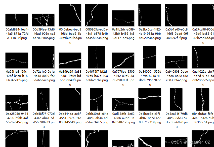
原始的项目结构我们如果想要套入自己的数据集的话只需要稍作改变即可,首先来看数据集:

标注数据如下所示:
接下来修改configs目录下config_setting.py模块,如下所示:
from torchvision import transforms
from utils import *

from datetime import datetime

class setting_config:
    """
    the config of training setting.
    """

    network = 'egeunet'
    model_config = {
        'num_classes': 1,
        'input_channels': 3,
        'c_list': [8,16,24,32,48,64],
        'bridge': True,
        'gt_ds': True,
    }

    datasets = 'isic18'
    if datasets == 'isic18':
        data_path = './data/isic2018/'
    elif datasets == 'isic17':
        data_path = './data/isic2017/'
    else:
        raise Exception('datasets in not right!')

    criterion = GT_BceDiceLoss(wb=1, wd=1)

    pretrained_path = './pre_trained/'
    num_classes = 1
    input_size_h = 256
    input_size_w = 256
    input_channels = 3
    distributed = False
    local_rank = -1
    num_workers = 0
    seed = 42
    world_size = None
    rank = None
    amp = False
    gpu_id = '0'
    batch_size = 192
    epochs = 100

    work_dir = 'results/' + network + '_' + datasets + '_' + datetime.now().strftime('%A_%d_%B_%Y_%Hh_%Mm_%Ss') + '/'

    print_interval = 20
    val_interval = 30
    save_interval = 10
    threshold = 0.5

    train_transformer = transforms.Compose([
        myNormalize(datasets, train=True),
        myToTensor(),
        myRandomHorizontalFlip(p=0.5),
        myRandomVerticalFlip(p=0.5),
        myRandomRotation(p=0.5, degree=[0, 360]),
        myResize(input_size_h, input_size_w)
    ])
    test_transformer = transforms.Compose([
        myNormalize(datasets, train=False),
        myToTensor(),
        myResize(input_size_h, input_size_w)
    ])

    opt = 'AdamW'
    assert opt in ['Adadelta', 'Adagrad', 'Adam', 'AdamW', 'Adamax', 'ASGD', 'RMSprop', 'Rprop', 'SGD'], 'Unsupported optimizer!'
    if opt == 'Adadelta':
        lr = 0.01 # default: 1.0 – coefficient that scale delta before it is applied to the parameters
        rho = 0.9 # default: 0.9 – coefficient used for computing a running average of squared gradients
        eps = 1e-6 # default: 1e-6 – term added to the denominator to improve numerical stability
        weight_decay = 0.05 # default: 0 – weight decay (L2 penalty)
    elif opt == 'Adagrad':
        lr = 0.01 # default: 0.01 – learning rate
        lr_decay = 0 # default: 0 – learning rate decay
        eps = 1e-10 # default: 1e-10 – term added to the denominator to improve numerical stability
        weight_decay = 0.05 # default: 0 – weight decay (L2 penalty)
    elif opt == 'Adam':
        lr = 0.001 # default: 1e-3 – learning rate
        betas = (0.9, 0.999) # default: (0.9, 0.999) – coefficients used for computing running averages of gradient and its square
        eps = 1e-8 # default: 1e-8 – term added to the denominator to improve numerical stability
        weight_decay = 0.0001 # default: 0 – weight decay (L2 penalty)
        amsgrad = False # default: False – whether to use the AMSGrad variant of this algorithm from the paper On the Convergence of Adam and Beyond
    elif opt == 'AdamW':
        lr = 0.001 # default: 1e-3 – learning rate
        betas = (0.9, 0.999) # default: (0.9, 0.999) – coefficients used for computing running averages of gradient and its square
        eps = 1e-8 # default: 1e-8 – term added to the denominator to improve numerical stability
        weight_decay = 1e-2 # default: 1e-2 – weight decay coefficient
        amsgrad = False # default: False – whether to use the AMSGrad variant of this algorithm from the paper On the Convergence of Adam and Beyond
    elif opt == 'Adamax':
        lr = 2e-3 # default: 2e-3 – learning rate
        betas = (0.9, 0.999) # default: (0.9, 0.999) – coefficients used for computing running averages of gradient and its square
        eps = 1e-8 # default: 1e-8 – term added to the denominator to improve numerical stability
        weight_decay = 0 # default: 0 – weight decay (L2 penalty)
    elif opt == 'ASGD':
        lr = 0.01 # default: 1e-2 – learning rate
        lambd = 1e-4 # default: 1e-4 – decay term
        alpha = 0.75 # default: 0.75 – power for eta update
        t0 = 1e6 # default: 1e6 – point at which to start averaging
        weight_decay = 0 # default: 0 – weight decay
    elif opt == 'RMSprop':
        lr = 1e-2 # default: 1e-2 – learning rate
        momentum = 0 # default: 0 – momentum factor
        alpha = 0.99 # default: 0.99 – smoothing constant
        eps = 1e-8 # default: 1e-8 – term added to the denominator to improve numerical stability
        centered = False # default: False – if True, compute the centered RMSProp, the gradient is normalized by an estimation of its variance
        weight_decay = 0 # default: 0 – weight decay (L2 penalty)
    elif opt == 'Rprop':
        lr = 1e-2 # default: 1e-2 – learning rate
        etas = (0.5, 1.2) # default: (0.5, 1.2) – pair of (etaminus, etaplis), that are multiplicative increase and decrease factors
        step_sizes = (1e-6, 50) # default: (1e-6, 50) – a pair of minimal and maximal allowed step sizes
    elif opt == 'SGD':
        lr = 0.01 # – learning rate
        momentum = 0.9 # default: 0 – momentum factor
        weight_decay = 0.05 # default: 0 – weight decay (L2 penalty)
        dampening = 0 # default: 0 – dampening for momentum
        nesterov = False # default: False – enables Nesterov momentum

    sch = 'CosineAnnealingLR'
    if sch == 'StepLR':
        step_size = epochs // 5 # – Period of learning rate decay.
        gamma = 0.5 # – Multiplicative factor of learning rate decay. Default: 0.1
        last_epoch = -1 # – The index of last epoch. Default: -1.
    elif sch == 'MultiStepLR':
        milestones = [60, 120, 150] # – List of epoch indices. Must be increasing.
        gamma = 0.1 # – Multiplicative factor of learning rate decay. Default: 0.1.
        last_epoch = -1 # – The index of last epoch. Default: -1.
    elif sch == 'ExponentialLR':
        gamma = 0.99 #  – Multiplicative factor of learning rate decay.
        last_epoch = -1 # – The index of last epoch. Default: -1.
    elif sch == 'CosineAnnealingLR':
        T_max = 50 # – Maximum number of iterations. Cosine function period.
        eta_min = 0.00001 # – Minimum learning rate. Default: 0.
        last_epoch = -1 # – The index of last epoch. Default: -1.
    elif sch == 'ReduceLROnPlateau':
        mode = 'min' # – One of min, max. In min mode, lr will be reduced when the quantity monitored has stopped decreasing; in max mode it will be reduced when the quantity monitored has stopped increasing. Default: ‘min’.
        factor = 0.1 # – Factor by which the learning rate will be reduced. new_lr = lr * factor. Default: 0.1.
        patience = 10 # – Number of epochs with no improvement after which learning rate will be reduced. For example, if patience = 2, then we will ignore the first 2 epochs with no improvement, and will only decrease the LR after the 3rd epoch if the loss still hasn’t improved then. Default: 10.
        threshold = 0.0001 # – Threshold for measuring the new optimum, to only focus on significant changes. Default: 1e-4.
        threshold_mode = 'rel' # – One of rel, abs. In rel mode, dynamic_threshold = best * ( 1 + threshold ) in ‘max’ mode or best * ( 1 - threshold ) in min mode. In abs mode, dynamic_threshold = best + threshold in max mode or best - threshold in min mode. Default: ‘rel’.
        cooldown = 0 # – Number of epochs to wait before resuming normal operation after lr has been reduced. Default: 0.
        min_lr = 0 # – A scalar or a list of scalars. A lower bound on the learning rate of all param groups or each group respectively. Default: 0.
        eps = 1e-08 # – Minimal decay applied to lr. If the difference between new and old lr is smaller than eps, the update is ignored. Default: 1e-8.
    elif sch == 'CosineAnnealingWarmRestarts':
        T_0 = 50 # – Number of iterations for the first restart.
        T_mult = 2 # – A factor increases T_{i} after a restart. Default: 1.
        eta_min = 1e-6 # – Minimum learning rate. Default: 0.
        last_epoch = -1 # – The index of last epoch. Default: -1.
    elif sch == 'WP_MultiStepLR':
        warm_up_epochs = 10
        gamma = 0.1
        milestones = [125, 225]
    elif sch == 'WP_CosineLR':
        warm_up_epochs = 20
可以看到:这里datasets我没有修改,数据集是直接在内容层面替换了isic2018的数据集,大家也可以这么做,当然了也可以再代码里面加入新的逻辑,比如:
datasets = 'self'
if datasets == 'isic18':
    data_path = './data/isic2018/'
elif datasets == 'isic17':
    data_path = './data/isic2017/'
elif datasets == "self":
    data_path = "/data/self/"
else:
    raise Exception('datasets in not right!')
我是不想麻烦,所以选择了直接数据替换的方式。
主要的配置参数如下:
pretrained_path = './pre_trained/'
num_classes = 1
input_size_h = 256
input_size_w = 256
input_channels = 3
distributed = False
local_rank = -1
num_workers = 0
seed = 42
world_size = None
rank = None
amp = False
gpu_id = '0'
batch_size = 192
epochs = 100

work_dir = 'results/' + network + '_' + datasets + '_' + datetime.now().strftime('%A_%d_%B_%Y_%Hh_%Mm_%Ss') + '/'

print_interval = 20
val_interval = 30
save_interval = 10
threshold = 0.5
官方默认是300个epoch的迭代计算,这里我为了节省时间修改为了100个epoch。
默认batch_size为8,这里我的显存比较大我修改为了192,可以根据自己的实际情况进行修改即可。
默认save_interval为100,这里因为我的总训练epoch就是100,所以我修改为了10,让模型训练过程中的存储频率更高点。
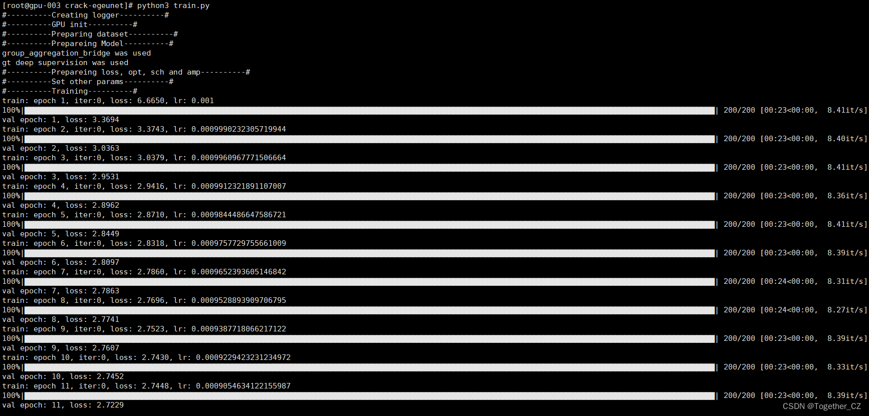
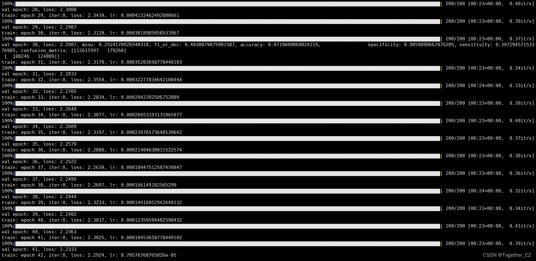
之后即可在终端执行train.py模块,输出如下所示:
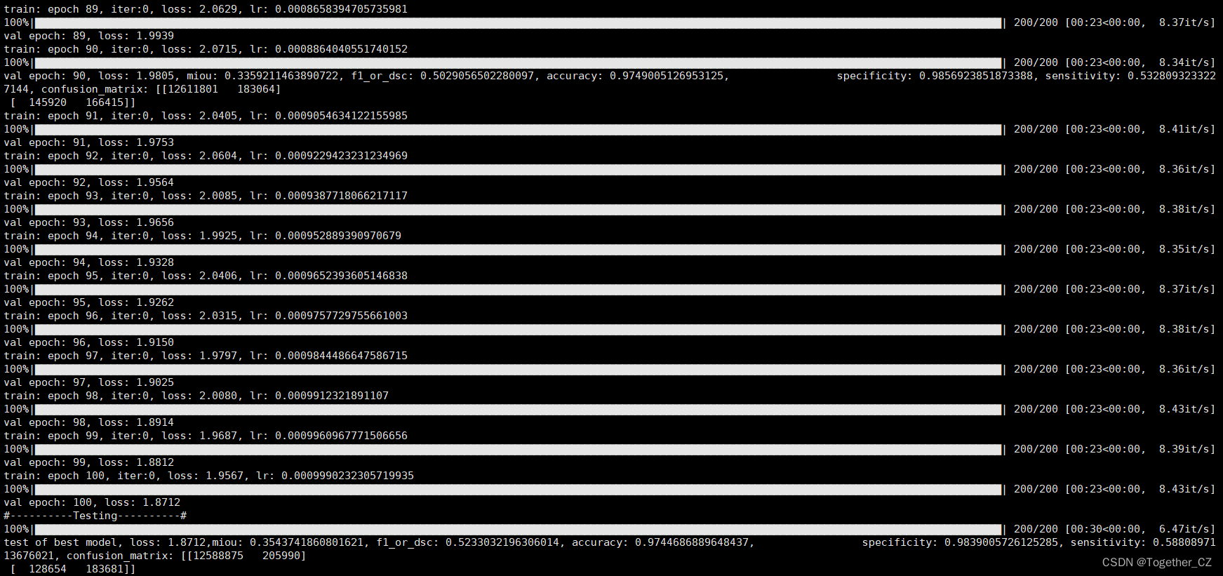
接下来看下outputs中存储的训练实例,如下所示:


这里看下实际可视化推理效果:
对比分割结果显示:

单独分割结果显示:
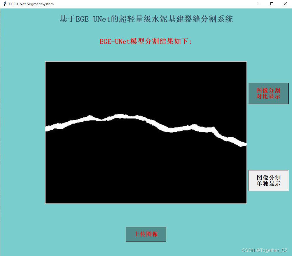
在推理时间消耗上面跟前文的医疗图像相比更长了一些,这个跟图像本身有关,医疗的数据集分辨率更低,不过这里单张图像的推理时耗相比于以往的模型依旧是很有优势的。
如果实际业务中有分割的相关需求都可以自行开发尝试下。