Van der Pol方程如下所示
d
x
d
t
=
y
d
y
d
t
=
−
x
+
(
1
−
x
2
)
y
\begin{equation} \begin{aligned} \frac{dx}{dt} & = y \\ \frac{dy}{dt} & = -x+(1-x^2)y \end{aligned} \end{equation}
dtdxdtdy=y=−x+(1−x2)y
相应的程序如下
为了观看长期趋势,将仿真时间定为100s
# 此脚本用以绘制Van der Pol微分方程的方向场

# 必要的包
import math
import matplotlib.pyplot as plt
import numpy as np
# 这里的x y应该是泛型的,既可以是标量也可以是向量也可以是矩阵
def diff_x(x, y):
    return y

def diff_y(x, y):
    return -x + (1 - x**2)*y;


x_cord = np.linspace(-3, 3, 10);
y_cord = x_cord;

X, Y = np.meshgrid(x_cord, y_cord);
U = diff_x(X, Y);
V = diff_y(X, Y);
# 归一化
N = np.sqrt(U ** 2 + V ** 2);
U = U / N;
V = V / N;

plt.quiver(X, Y, U, V, color='r');

# 画一个解的曲线
x0 = np.array([-3,-2.5, -2.7, 3, 3, -0.1]);
y0 = np.array([-3, 3, 3, 3, -3, 0]);

delta_t = 0.05;
time = np.arange(0, 100+delta_t, delta_t);
x_sol = np.zeros([len(x0), len(time)]); # 5行 几百列
y_sol = np.zeros([len(y0), len(time)]);


for i in range(len(time)):
    if i == 0:
        x_sol[:,i] = x0;
        y_sol[:,i] = y0;
    else:
        x_sol[:,i] = x_sol[:,i-1] + diff_x(x_sol[:,i-1], y_sol[:,i-1]) * delta_t;
        y_sol[:,i] = y_sol[:,i-1] + diff_y(x_sol[:,i-1], y_sol[:,i-1]) * delta_t;

for j in range(len(x0)):
    plt.plot(x_sol[j,:], y_sol[j,:]);
plt.title(r"$Direction\  Field\  of\  Van\  der\  Pol\  system$");
plt.xlabel(r"$x$");
plt.ylabel(r"$y$");
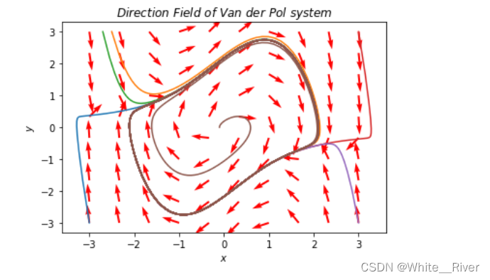
Van der Pol方程是一个非线性方程, 对于非线性方程, 我们目前还没有通用的工具分析, 但如果把比例尺放大, 只在平衡点附近观察, 更细致地观看平衡点(0,0)附近, 同时缩小仿真仿真的时间,我们会发现平衡点附近该方程的行为有点像线性系统中的spiral source 也就是二阶线性系统的不稳定焦点
这也给了我们一个启示, 即可以在平衡点附近, 在较小的时间间隔内, 把非线性系统看做线性系统
以下就是系统在平衡点附近的行为
仿真时间减小为10s
x y坐标缩小到±0.3
代码如下
x_cord = np.linspace(-0.3, 0.3, 10);
y_cord = x_cord;

X, Y = np.meshgrid(x_cord, y_cord);
U = diff_x(X, Y);
V = diff_y(X, Y);
# 归一化
N = np.sqrt(U ** 2 + V ** 2);
U = U / N;
V = V / N;

plt.quiver(X, Y, U, V, color='r');


# 画一个解的曲线
x0 = np.linspace(-0.001,0.001, 5);
y0 = x0;

delta_t = 0.005;
time = np.arange(0, 10.5+delta_t, delta_t);
x_sol = np.zeros([len(x0), len(time)]); # 5行 几百列
y_sol = np.zeros([len(y0), len(time)]);


for i in range(len(time)):
    if i == 0:
        x_sol[:,i] = x0;
        y_sol[:,i] = y0;
    else:
        x_sol[:,i] = x_sol[:,i-1] + diff_x(x_sol[:,i-1], y_sol[:,i-1]) * delta_t;
        y_sol[:,i] = y_sol[:,i-1] + diff_y(x_sol[:,i-1], y_sol[:,i-1]) * delta_t;

for j in range(len(x0)):
    plt.plot(x_sol[j,:], y_sol[j,:]);
plt.title(r"$Direction\  Field\  of\  Van\  der\  Pol\  system$");
plt.xlabel(r"$x$");
plt.ylabel(r"$y$");
如图所示
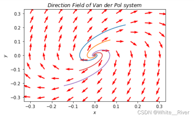
这个就很像二阶系统的不稳定焦点


![[SUCTF2019]hardcpp](https://img-blog.csdnimg.cn/da3dc2aaccda4feab625cd1b998a7ca9.png)