目录
- Topic Modelling
- A Brief History of Topic Models
- LDA
- Evaluation
- Conclusion
Topic Modelling
-
makeingsense of text
- English Wikipedia: 6M articles
- Twitter: 500M tweets per day
- New York Times: 15M articles
- arXiv: 1M articles
- What can we do if we want to learn something about these document collections?
-
questions
- What are the less popular topics on Wikipedia?
- What are the big trends on Twitter in the past month?
- How do the social issues evolve over time in New York Times from 1900s to 2000s?
- What are some influential research areas?
-
topic models to the rescue
- Topic models learn common, overlapping themes in a document collection
- Unsupervised model
- No labels; input is just the documents!
- What’s the output of a topic model?
- Topics: each topic associated with a list of words
- Topic assignments: each document associated with a list of topics
-
what do topics look like
-
A list of words
-
Collectively describes a concept or subject
-
Words of a topic typically appear in the same set of documents in the corpus(words overlapping in documents)

-
Wikipedia topics(broad)

-
Twitter topics(short,conversational)

-
New York Times topics

-
-
applications of topic models
- Personalised advertising(e.g. types of products bought)
- Search engine
- Discover senses of polysemous words(e.g. apple: fruit, company, two different clusters)
A Brief History of Topic Models
-
latent semantic analysis

-
LSA: truncate

-
issues
- Positive and negative values in the U U U and V T V^T VT
- Difficult to interpret(negative values)

-
-
probabilistic LSA
-
based on a probabilistic model to get rid of negative values

-
issues
- No more negative values!
- PLSA can learn topics and topic assignment for documents in the train corpus
- But it is unable to infer topic distribution on new documents
- PLSA needs to be re-trained for new documents
-
-
latent dirichlet allocation(LDA)
- Introduces a prior to the document-topic and topicword distribution
- Fully generative: trained LDA model can infer topics on unseen documents!
- LDA is a Bayesian version of PLSA
LDA
-
LDA
- Core idea: assume each document contains a mix of topics
- But the topic structure is hidden (latent)
- LDA infers the topic structure given the observed words and documents
- LDA produces soft clusters of documents (based on topic overlap), rather than hard clusters
- Given a trained LDA model, it can infer topics on new documents (not part of train data)

-
input
- A collection of documents
- Bag-of-words
- Good preprocessing practice:
- Remove stopwords
- Remove low and high frequency word types
- Lemmatisation
-
output
-
Topics: distribution over words in each topic

-
Topic assignment: distribution over topics in each document

-
-
learning
-
How do we learn the latent topics?
-
Two main family of algorithms:
- Variational methods
- Sampling-based methods
-
sampling method (Gibbs)
-
Randomly assign topics to all tokens in documents

-
Collect topic-word and document-topic co-occurrence statistics based on the assignments
-
first give some psudo-counts in every cell of two matrix(smoothing,no event is 0)

-
collect co-occurrence statistics

-
-
Go through every word token in corpus and sample a new topic:
-
delete current topic assigned to a word

-
update two matrices

-
compute the probability distribution to sample: P ( t i ∣ w , d ) ∝ P ( t i ∣ w ) P ( t i ∣ d ) P(t_i|w,d) \propto P(t_i|w)P(t_i|d) P(ti∣w,d)∝P(ti∣w)P(ti∣d) ( P ( t i ∣ w ) → P(t_i|w) \to P(ti∣w)→ topic-word, P ( t i ∣ d ) → P(t_i|d) \to P(ti∣d)→ document-topic)

- P ( t 1 ∣ w , d ) = P ( t 1 ∣ m o u s e ) × P ( t 1 ∣ d 1 ) = 0.01 0.01 + 0.01 + 2.01 × 1.1 1.1 + 1.1 + 2.1 P(t_1|w,d)=P(t_1|mouse)\times{P(t_1|d_1)}=\frac{0.01}{0.01+0.01+2.01}\times{\frac{1.1}{1.1+1.1+2.1}} P(t1∣w,d)=P(t1∣mouse)×P(t1∣d1)=0.01+0.01+2.010.01×1.1+1.1+2.11.1
-
sample randomly based on the probability distribution
-
-
Go to step 2 and repeat until convergence
- when to stop
- Train until convergence
- Convergence = model probability of training set becomes stable
- How to compute model probability?
- l o g P ( w 1 , w 2 , . . . , w m ) = l o g ∑ j = 0 T P ( w 1 ∣ t j ) P ( t j ∣ d w 1 ) + . . . + l o g ∑ j = 0 T P ( w m ∣ t j ) P ( t j ∣ d w m ) logP(w_1,w_2,...,w_m)=log\sum_{j=0}^TP(w_1|t_j)P(t_j|d_{w_1})+...+log\sum_{j=0}^TP(w_m|t_j)P(t_j|d_{w_m}) logP(w1,w2,...,wm)=log∑j=0TP(w1∣tj)P(tj∣dw1)+...+log∑j=0TP(wm∣tj)P(tj∣dwm)
- m = #word tokens
- P ( w 1 ∣ t j ) → P(w_1|t_j) \to P(w1∣tj)→ based on the topic-word co-occurrence matrix
- P ( t j ∣ d w 1 ) → P(t_j|d_{w_1}) \to P(tj∣dw1)→ based on the document-topic co-occurrence matrix
- infer topics for new documents
-
Randomly assign topics to all tokens in new/test documents

-
Update document-topic matrix based on the assignments; but use the trained topic-word matrix (kept fixed)

-
Go through every word in the test documents and sample topics: P ( t i ∣ w , d ) ∝ P ( t i ∣ w ) P ( t i ∣ d ) P(t_i|w,d) \propto P(t_i|w)P(t_i|d) P(ti∣w,d)∝P(ti∣w)P(ti∣d)
-
Go to step 2 and repeat until convergence
-
- hyper-parameters
-
T T T: number of topic

-
β \beta β: prior on the topic-word distribution
-
α \alpha α: prior on the document-topic distribution
-
Analogous to k in add-k smoothing in N-gram LM
-
Pseudo counts to initialise co-occurrence matrix:

-
High prior values → \to → flatter distribution

- a very very large value would lead to a uniform distribution
-
Low prior values → \to → peaky distribution

-
β \beta β: generally small (< 0.01)
- Large vocabulary, but we want each topic to focus on specific themes
-
α \alpha α: generally larger (> 0.1)
- Multiple topics within a document
-
-
-
Evaluation
- how to evaluate topic models
- Unsupervised learning → \to → no labels
- Intrinsic(内在的,固有的) evaluation:
- model logprob / perplexity(困惑度,复杂度) on test documents
- l o g L = ∑ W ∑ T l o g P ( w ∣ t ) P ( t ∣ d w ) logL=\sum_W\sum_TlogP(w|t)P(t|d_w) logL=∑W∑TlogP(w∣t)P(t∣dw)
- p p l = e x p − l o g L W ppl=exp^{\frac{-logL}{W}} ppl=expW−logL
- issues with perlexity
- More topics = better (lower) perplexity
- Smaller vocabulary = better perplexity
- Perplexity not comparable for different corpora, or different tokenisation/preprocessing methods
- Does not correlate with human perception of topic quality
- Extrinsic(外在的) evaluation the way to go:
- Evaluate topic models based on downstream task
- topic coherence
-
A better intrinsic evaluation method
-
Measure how coherent the generated topics (blue more coherent than red)

-
A good topic model is one that generates more coherent topics
-
- word intrusion
- Idea: inject one random word to a topic
- {farmers, farm, food, rice, agriculture} → \to → {farmers, farm, food, rice, cat, agriculture}
- Ask users to guess which is the intruder word
- Correct guess → \to → topic is coherent
- Try guess the intruder word in:
- {choice, count, village, i.e., simply, unionist}
- Manual effort; does not scale
- Idea: inject one random word to a topic
- PMI
≈
\approx
≈ coherence?
- High PMI for a pair of words
→
\to
→ words are correlated
- PMI(farm, rice) ↑ \uparrow ↑
- PMI(choice, village) ↓ \downarrow ↓
- If all word pairs in a topic has high PMI → \to → topic is coherent
- If most topics have high PMI → \to → good topic model
- Where to get word co-occurrence statistics for PMI?
- Can use same corpus for topic model
- A better way is to use an external corpus (e.g. Wikipedia)
- High PMI for a pair of words
→
\to
→ words are correlated
- PMI
- Compute pairwise PMI of top-N words in a topic
- P M I ( t ) = ∑ j = 2 N ∑ i = 1 j − 1 l o g P ( w i , w j ) P ( w i ) P ( w j ) PMI(t)=\sum_{j=2}^N\sum_{i=1}^{j-1}log\frac{P(w_i,w_j)}{P(w_i)P(w_j)} PMI(t)=∑j=2N∑i=1j−1logP(wi)P(wj)P(wi,wj)
- Given topic: {farmers, farm, food, rice, agriculture}
- Coherence = sum PMI for all word pairs:
- PMI(farmers, farm) + PMI(farmers, food) + … + PMI(rice, agriculture)
- variants
- Normalised PMI
- N P M I ( t ) = ∑ j = 2 N ∑ i = 1 j − 1 l o g P ( w i , w j ) P ( w i ) P ( w j ) − l o g P ( w i , w j ) NPMI(t)=\sum_{j=2}^N\sum_{i=1}^{j-1}\frac{log\frac{P(w_i,w_j)}{P(w_i)P(w_j)}}{-logP(w_i,w_j)} NPMI(t)=∑j=2N∑i=1j−1−logP(wi,wj)logP(wi)P(wj)P(wi,wj)
- conditional probability (proved not as good as PMI)
- L C P ( t ) = ∑ j = 2 N ∑ i = 1 j − 1 l o g P ( w i , w j ) P ( w i ) LCP(t)=\sum_{j=2}^N\sum_{i=1}^{j-1}log\frac{P(w_i,w_j)}{P(w_i)} LCP(t)=∑j=2N∑i=1j−1logP(wi)P(wi,wj)
- Normalised PMI
- example (PMI tends to favor rarer words, use NPMI to relieve this problem)
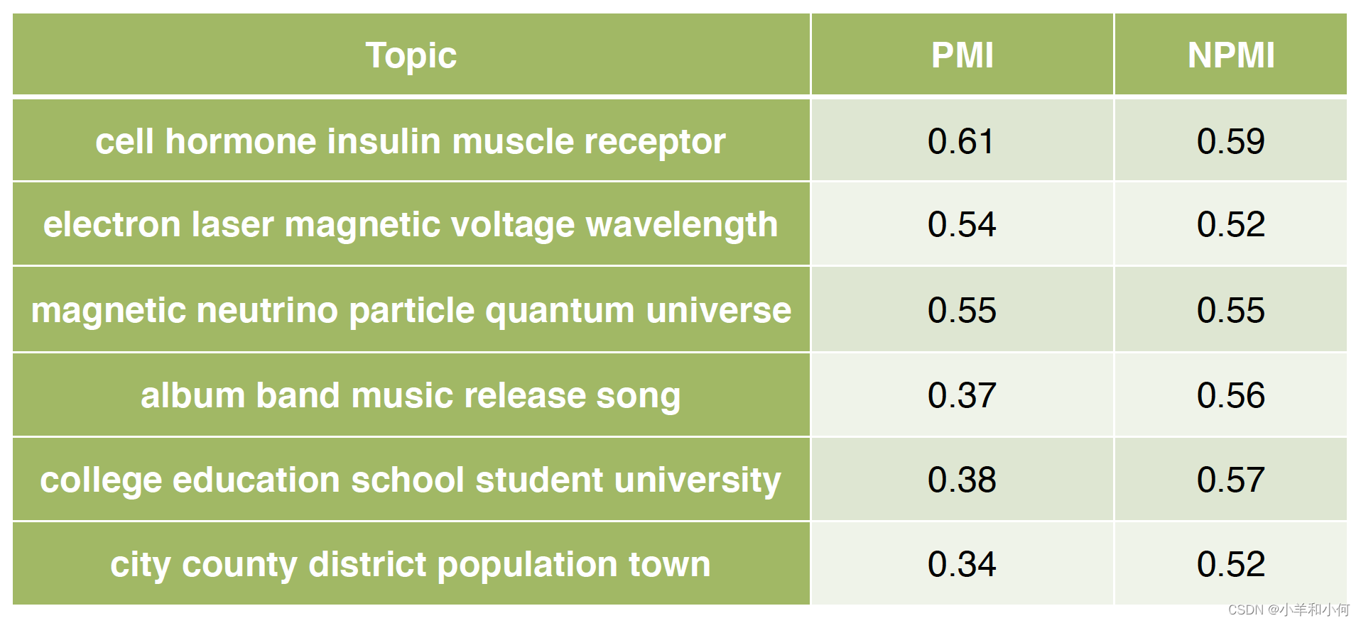
- Compute pairwise PMI of top-N words in a topic
Conclusion
- Topic model: an unsupervised model for learning latent concepts in a document collection
- LDA: a popular topic model
- Learning
- Hyper-parameters
- How to evaluate topic models?
- Topic coherence