桓峰基因公众号推出单细胞生信分析教程并配有视频在线教程,目前整理出来的相关教程目录如下:
Topic 6. 克隆进化之 Canopy
Topic 7. 克隆进化之 Cardelino
Topic 8. 克隆进化之 RobustClone
SCS【1】今天开启单细胞之旅,述说单细胞测序的前世今生
SCS【2】单细胞转录组 之 cellranger
SCS【3】单细胞转录组数据 GEO 下载及读取
SCS【4】单细胞转录组数据可视化分析 (Seurat 4.0)
SCS【5】单细胞转录组数据可视化分析 (scater)
SCS【6】单细胞转录组之细胞类型自动注释 (SingleR)
SCS【7】单细胞转录组之轨迹分析 (Monocle 3) 聚类、分类和计数细胞
SCS【8】单细胞转录组之筛选标记基因 (Monocle 3)
SCS【9】单细胞转录组之构建细胞轨迹 (Monocle 3)
SCS【10】单细胞转录组之差异表达分析 (Monocle 3)
SCS【11】单细胞ATAC-seq 可视化分析 (Cicero)
SCS【12】单细胞转录组之评估不同单细胞亚群的分化潜能 (Cytotrace)
SCS【13】单细胞转录组之识别细胞对“基因集”的响应 (AUCell)
SCS【14】单细胞调节网络推理和聚类 (SCENIC)
SCS【15】细胞交互:受体-配体及其相互作用的细胞通讯数据库 (CellPhoneDB)
SCS【16】从肿瘤单细胞RNA-Seq数据中推断拷贝数变化 (inferCNV)
SCS【17】从单细胞转录组推断肿瘤的CNV和亚克隆 (copyKAT)
SCS【18】细胞交互:受体-配体及其相互作用的细胞通讯数据库 (iTALK)
SCS【19】单细胞自动注释细胞类型 (Symphony)
SCS【20】单细胞数据估计组织中细胞类型(Music)
SCS【21】单细胞空间转录组可视化 (Seurat V5)
SCS【22】单细胞转录组之 RNA 速度估计 (Velocyto.R)
SCS【23】单细胞转录组之数据整合 (Harmony)
SCS【24】单细胞数据量化代谢的计算方法 (scMetabolism)
SCS【25】单细胞细胞间通信第一部分细胞通讯可视化(CellChat)
SCS【26】单细胞细胞间通信第二部分通信网络的系统分析(CellChat)
简 介
单细胞RNA测序(scRNA-seq)是一种广泛应用于分析单个细胞中基因表达的技术。这使得分子生物学可以在细胞群体的大量测序无法匹配的分辨率下进行研究。scran软件包实现了对scRNA-seq数据进行低级处理的方法,包括细胞周期相位分配、方差建模以及标记基因和基因相关性的测试。
注意:在scRNA-seq分析工作流程中使用scran(以及其他包)的更全面的描述可在 https://osca.bioconductor.org 获得。
软件包安装
if (!requireNamespace("BiocManager", quietly = TRUE))
  install.packages("BiocManager")

BiocManager::install("scran")
数据读取
从一个计数矩阵开始,每一行是一个基因,每一列是一个细胞。这些可以通过将读取序列映射到参考基因组,然后计算映射到每个基因外显子的读取数来获得。(例如,请参阅完成这两项任务的Rsubread包。)或者,伪比对方法可用于量化每个细胞中每个转录本的丰度。为简单起见,我们将从scRNAseq包中提取一个现有的数据集。
library(scran)
library(scRNAseq)
sce <- GrunPancreasData()
sce
## class: SingleCellExperiment
## dim: 20064 1728
## metadata(0):
## assays(1): counts
## rownames(20064): A1BG-AS1__chr19 A1BG__chr19 ... ZZEF1__chr17
##   ZZZ3__chr1
## rowData names(2): symbol chr
## colnames(1728): D2ex_1 D2ex_2 ... D17TGFB_95 D17TGFB_96
## colData names(2): donor sample
## reducedDimNames(0):
## mainExpName: endogenous
## altExpNames(1): ERCC
该数据集来自 CEL-seq 对人类胰腺进行的研究(Grun et al. 2016)。作为 SingleCellExperiment 对象提供,其中包含原始数据和各种注释。只需要进行一些粗略的质量控制,以去除总计数低或峰值百分比高的细胞:
library(scuttle)
qcstats <- perCellQCMetrics(sce)
qcfilter <- quickPerCellQC(qcstats, percent_subsets = "altexps_ERCC_percent")
sce <- sce[, !qcfilter$discard]
summary(qcfilter$discard)
##    Mode   FALSE    TRUE
## logical    1291     437
使用 computeSumFactors 方法对细胞特异性偏差进行归一化,该方法实现了缩放归一化的反卷积策略:
library(scran)
clusters <- quickCluster(sce)
sce <- computeSumFactors(sce, clusters = clusters)
summary(sizeFactors(sce))
##     Min.  1st Qu.   Median     Mean  3rd Qu.     Max.
## 0.006722 0.442629 0.801312 1.000000 1.295809 9.227575
sce <- logNormCounts(sce)
View(sce)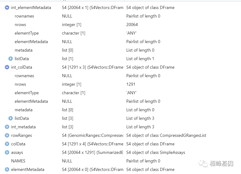
例子实操
差异建模(Variance modelling)
通过模拟每个基因的变异来识别驱动数据集中生物异质性的基因。通过在聚类等下游分析中仅使用高度可变基因的子集,去除由技术噪声驱动的无意义基因来提高生物结构的分辨率。通过拟合内源性方差的趋势,将每个基因的总方差分解为其生物和技术成分。
趋势的拟合值被用作技术分量的估计,从总方差中减去拟合值,得到每个基因的生物分量。
dec <- modelGeneVar(sce)
plot(dec$mean, dec$total, xlab = "Mean log-expression", ylab = "Variance")
curve(metadata(dec)$trend(x), col = "blue", add = TRUE)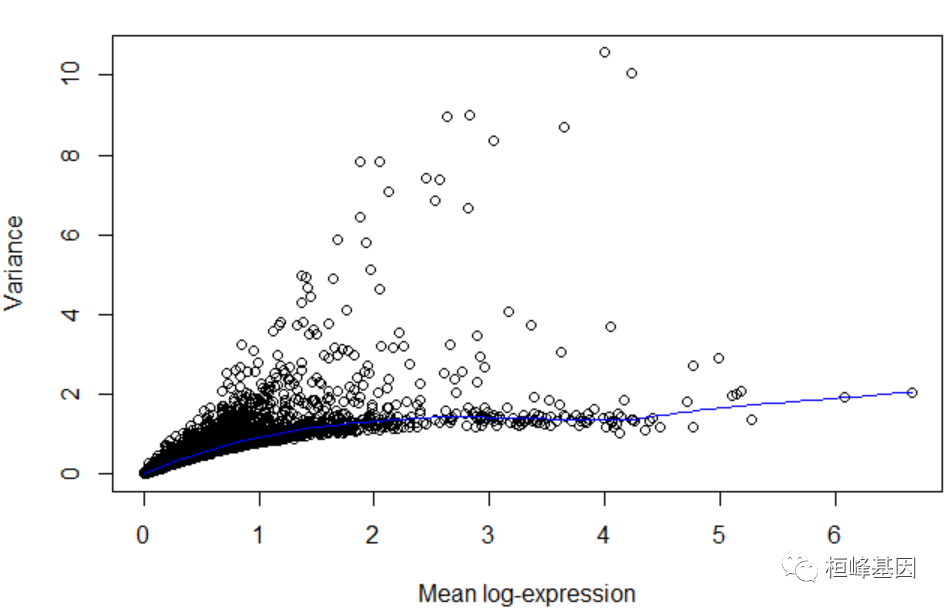
如果使用spike-ins来适应趋势。这为技术变异提供了更直接的估计,避免了大多数基因不表现出生物变异的假设:
dec2 <- modelGeneVarWithSpikes(sce, "ERCC")
plot(dec2$mean, dec2$total, xlab = "Mean log-expression", ylab = "Variance")
points(metadata(dec2)$mean, metadata(dec2)$var, col = "red")
curve(metadata(dec2)$trend(x), col = "blue", add = TRUE)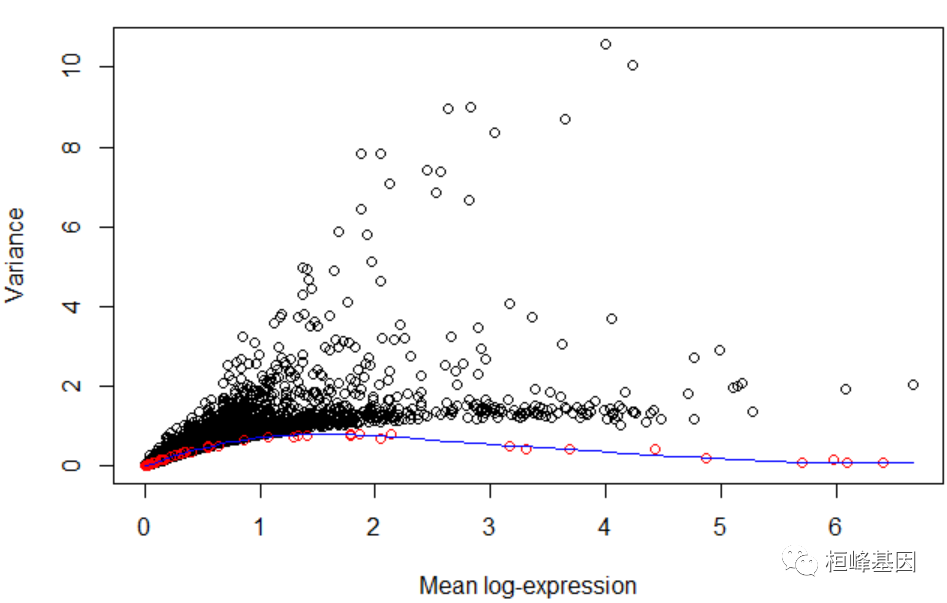
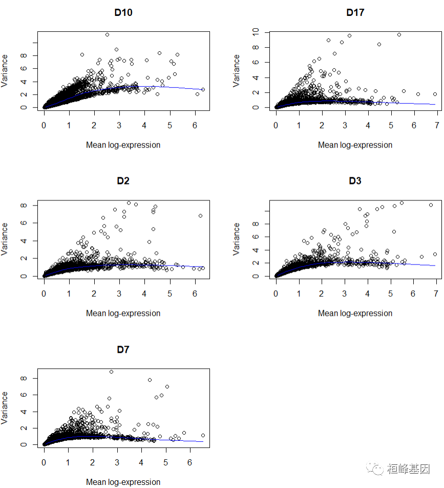
如果有一些无趣的变化因素,我们可以使用block=来屏蔽它们。这将在每个块内执行趋势拟合和分解,然后将跨块的统计数据组合以输出。还可以提取每个单独块的统计数据以供进一步检查。
# Turned off weighting to avoid overfitting for each donor.
dec3 <- modelGeneVar(sce, block = sce$donor, density.weights = FALSE)
per.block <- dec3$per.block
par(mfrow = c(3, 2))
for (i in seq_along(per.block)) {
    decX <- per.block[[i]]
    plot(decX$mean, decX$total, xlab = "Mean log-expression", ylab = "Variance",
        main = names(per.block)[i])
    curve(metadata(decX)$trend(x), col = "blue", add = TRUE)
}
然后,可以使用 getTopHVGs() 函数提取一些顶级基因用于下游分析。可以使用各种不同的策略来定义一个有趣的基因子集:
# Get the top 10% of genes.
top.hvgs <- getTopHVGs(dec, prop = 0.1)

# Get the top 2000 genes.
top.hvgs2 <- getTopHVGs(dec, n = 2000)

# Get all genes with positive biological components.
top.hvgs3 <- getTopHVGs(dec, var.threshold = 0)

# Get all genes with FDR below 5%.
top.hvgs4 <- getTopHVGs(dec, fdr.threshold = 0.05)
然后,被选择的基因子集可以传递给子集。在下游步骤中的subset.row参数。下面是PCA步骤的演示过程:
sce <- fixedPCA(sce, subset.row = top.hvgs)
reducedDimNames(sce)
## [1] "PCA"
自动化选项
主成分分析通常在下游分析之前进行降噪和压缩数据。一个常见的问题是要保留多少个人电脑;更多的个人电脑将捕获更多的生物信号,代价是保留更多的噪音和需要更多的计算工作。选择pc数量的一种方法是使用技术组件估计来确定应该保留的方差比例。
sced <- denoisePCA(sce, dec2, subset.row = getTopHVGs(dec2, prop = 0.1))
ncol(reducedDim(sced, "PCA"))
## [1] 50
另一种方法是基于这样的假设,即每个亚种群应该在不同的变异轴上彼此分离。因此,我们选择的pc数量不少于子种群的数量(当然,子种群的数量是未知的,因此我们使用集群的数量作为代理)。然后,将降维结果子集化到所需的pc数量是一件简单的事情。
output <- getClusteredPCs(reducedDim(sce))
npcs <- metadata(output)$chosen
reducedDim(sce, "PCAsub") <- reducedDim(sce, "PCA")[, 1:npcs, drop = FALSE]
npcs
## [1] 14
基于图论聚类
scRNA-seq数据的聚类通常使用基于图的方法进行,因为它们具有相对的可扩展性和鲁棒性。scran通过buildSNNGraph()函数提供了几种基于共享近邻的图构建方法。这通常是从选定的pc中生成的,之后可以使用来自igraph包的社区检测方法来显式地识别集群。
# In this case, using the PCs that we chose from getClusteredPCs().
g <- buildSNNGraph(sce, use.dimred = "PCAsub")
cluster <- igraph::cluster_walktrap(g)$membership

# Assigning to the 'colLabels' of the 'sce'.
colLabels(sce) <- factor(cluster)
table(colLabels(sce))
##
##   1   2   3   4   5   6   7   8   9  10  11  12
##  79 285  64 170 166 164 124  32  57  63  63  24
library(scater)
sce <- runTSNE(sce, dimred = "PCAsub")
plotTSNE(sce, colour_by = "label", text_by = "label")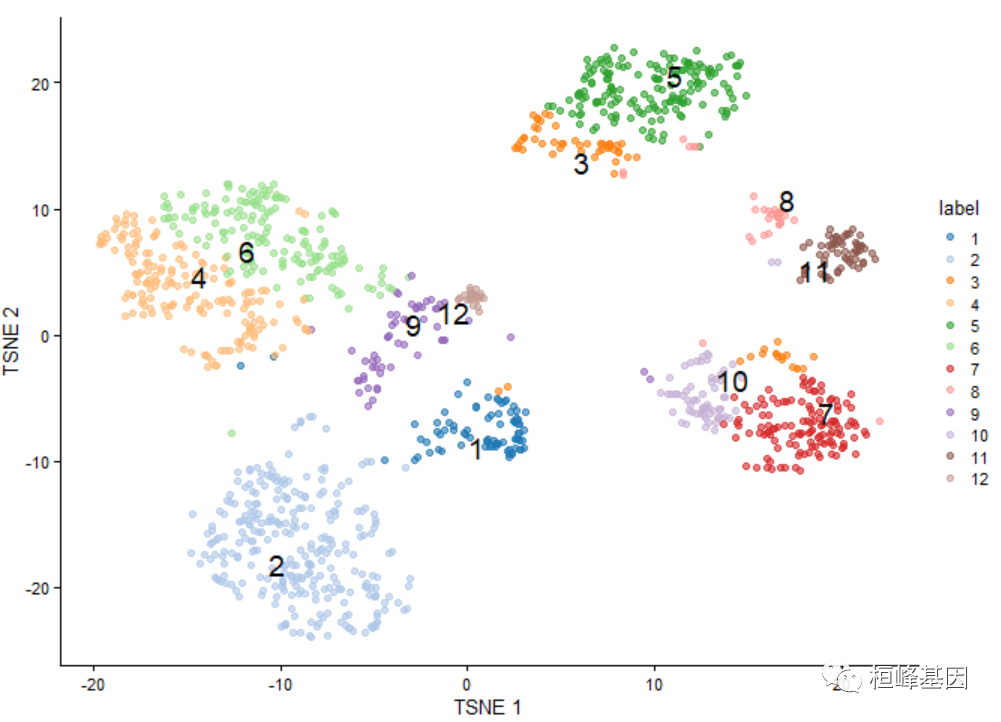
对于基于图的方法,另一种诊断方法是检查每对聚类的观察到的与期望的边权的比率(与许多cluster_*函数中使用的模块化分数密切相关)。通常期望看到同一簇中的单元之间的观察权重很高,而簇之间的权重最小,这表明簇之间的分离很好。非对角线条目表明一些集群是密切相关的,这对于检查它们是否被一致地注释是很有用的。
library(bluster)
ratio <- pairwiseModularity(g, cluster, as.ratio = TRUE)

library(pheatmap)
pheatmap(log10(ratio + 1), cluster_cols = FALSE, cluster_rows = FALSE, col = rev(heat.colors(100)))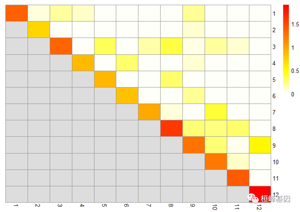
更一般的诊断包括启动,以确定集群之间分区的稳定性。给定一个聚类函数,bootstrapCluster()函数使用自举计算每对原始集群的共分配概率,即从每个集群中随机选择一个单元格在自举复制中被分配到同一集群的概率。较大的概率表明,这些聚类之间的分离在一定程度上是不稳定的,它对采样噪声敏感,因此不应用于下游推断。
ass.prob <- bootstrapStability(sce, FUN = function(x) {
    g <- buildSNNGraph(x, use.dimred = "PCAsub")
    igraph::cluster_walktrap(g)$membership
}, clusters = sce$cluster)

pheatmap(ass.prob, cluster_cols = FALSE, cluster_rows = FALSE, col = colorRampPalette(c("white",
    "blue"))(100))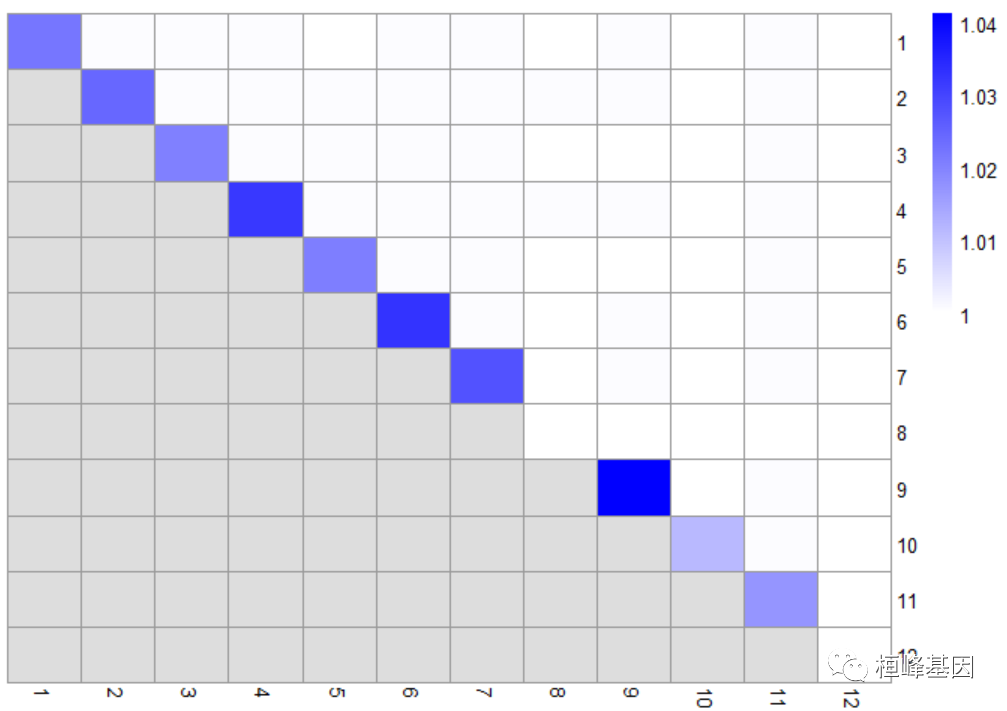
subout <- quickSubCluster(sce, groups = colLabels(sce))
table(metadata(subout)$subcluster)  # formatted as '<parent>.<subcluster>'
##
##  1.1  1.2 10.1 10.2 10.3 11.1 11.2   12  2.1  2.2  2.3  2.4  3.1  3.2  3.3  4.1
##   38   41   16   19   28   29   34   24   96   35   81   73   26   19   19   53
##  4.2  4.3  4.4  5.1  5.2  6.1  6.2  6.3  7.1  7.2  7.3    8  9.1  9.2
##   67   33   17   73   93   64   65   35   35   35   54   32   33   24
识别标记基因
scoreMarkers()包装函数将执行集群对之间的差异表达比较,以识别潜在的标记基因。
# Uses clustering information from 'colLabels(sce)' by default:
markers <- scoreMarkers(sce)
markers
## List of length 12
## names(12): 1 2 3 4 5 6 7 8 9 10 11 12
快速总结cluster1的最佳标记基因:
markers[[1]][order(markers[[1]]$mean.AUC, decreasing = TRUE), 1:4]
## DataFrame with 20064 rows and 4 columns
##                 self.average other.average self.detected other.detected
##                    <numeric>     <numeric>     <numeric>      <numeric>
## UGDH-AS1__chr4       7.95736       2.97892      1.000000       0.916095
## KCNQ1OT1__chr11      8.63439       3.86267      1.000000       0.977219
## PGM5P2__chr9         5.93842       1.37177      0.987342       0.629164
## MAB21L3__chr1        6.52394       2.07597      0.987342       0.808723
## FBLIM1__chr1         5.05717       1.39738      0.987342       0.700471
## ...                      ...           ...           ...            ...
## SKP1__chr5          0.526165       1.91257      0.329114       0.827098
## EIF1__chr17         1.453564       3.41013      0.506329       0.943458
## RPL3__chr22         1.606360       3.67678      0.544304       0.963845
## RPS25__chr11        1.400783       3.43745      0.493671       0.962767
## GNAS__chr20         1.295445       3.99483      0.493671       0.941651
返回数据框:
markers <- scoreMarkers(sce, full.stats = TRUE)
markers[[1]]$full.logFC.cohen
## DataFrame with 20064 rows and 11 columns
##                         2          3         4          5         6          7
##                 <numeric>  <numeric> <numeric>  <numeric> <numeric>  <numeric>
## A1BG-AS1__chr19  0.193192   0.193192  0.193192  0.1511082  0.193192  0.1931922
## A1BG__chr19     -0.383283  -0.810316  0.012951 -1.1128084  0.162714 -1.0253400
## A1CF__chr10     -0.150129  -0.553733  0.451479 -0.7289524  0.361270  0.1736118
## A2M-AS1__chr12   0.185977  -0.119582  0.277078  0.0826094  0.277078  0.0205016
## A2ML1__chr12     0.492297   0.348947  0.528591  0.5659760  0.554566  0.5659760
## ...                   ...        ...       ...        ...       ...        ...
## ZYG11A__chr1     0.618620  0.5733540  0.539024   0.644377  0.681953   0.681953
## ZYG11B__chr1     1.535652  1.1280983  1.391627   1.756829  1.601884   1.659232
## ZYX__chr7       -0.221250  0.2823101 -0.349240   0.238468 -0.589359   0.295469
## ZZEF1__chr17    -0.509875 -0.0383699 -0.375748  -0.388188 -0.394200  -0.640098
## ZZZ3__chr1      -0.433631 -0.2503621 -0.341861  -0.361327 -0.344299  -0.522964
##                         8          9        10         11        12
##                 <numeric>  <numeric> <numeric>  <numeric> <numeric>
## A1BG-AS1__chr19  0.193192 -0.0847779  0.193192  0.1931922  0.193192
## A1BG__chr19     -0.960358  0.2744821 -0.929347 -0.7301001 -1.356154
## A1CF__chr10     -0.327091  0.1862410  0.390848 -0.2785467  0.570966
## A2M-AS1__chr12   0.277078  0.2770778 -0.105477 -0.0741515  0.277078
## A2ML1__chr12     0.525356  0.4527881  0.493265  0.5659760  0.565976
## ...                   ...        ...       ...        ...       ...
## ZYG11A__chr1     0.681953  0.3991683  0.681953   0.616473  0.593276
## ZYG11B__chr1     1.714765  1.3265656  1.539204   1.579707  1.574035
## ZYX__chr7        0.329949  0.0333088  0.155112   0.299053 -1.385087
## ZZEF1__chr17    -0.380311 -0.1101065 -0.614079  -0.544608 -0.370839
## ZZZ3__chr1      -0.183771 -0.3009860 -0.440704  -0.433413 -0.321751
检测相关基因
另一个有用的方法是确定HVGs 对之间显著的两两相关性。这个想法是为了区分由随机随机性引起的HVGs 和那些驱动系统异质性的HVGs ,例如亚种群之间的HVGs 。相关性由correlatePairs方法计算,该方法使用稍微修改过的Spearman 's rho,并使用cor.test()中相同的方法对零相关性的零假设进行检验。
# Using the first 200 HVs, which are the most interesting anyway.
of.interest <- top.hvgs[1:200]
cor.pairs <- correlatePairs(sce, subset.row = of.interest)
cor.pairs
## DataFrame with 19900 rows and 5 columns
##                 gene1          gene2          rho      p.value          FDR
##           <character>    <character>    <numeric>    <numeric>    <numeric>
## 1     KCNQ1OT1__chr11 UGDH-AS1__chr4     0.830625  0.00000e+00  0.00000e+00
## 2           CPE__chr4    SCG5__chr15     0.813664 6.05366e-306 6.02339e-302
## 3         CHGA__chr14    SCG5__chr15     0.808313 7.64265e-299 5.06963e-295
## 4           GCG__chr2     TTR__chr18     0.803692 6.86304e-293 3.41436e-289
## 5         CHGB__chr20      CPE__chr4     0.802498 2.23623e-291 8.90020e-288
## ...               ...            ...          ...          ...          ...
## 19896      ELF3__chr1 METTL21A__chr2  3.83996e-05     0.998900     0.999101
## 19897      EGR1__chr5    NPTX2__chr7 -2.94559e-05     0.999156     0.999307
## 19898     ODF2L__chr1      VGF__chr7 -2.25268e-05     0.999355     0.999455
## 19899 LOC90834__chr22  SLC30A8__chr8  1.99362e-05     0.999429     0.999479
## 19900       IL8__chr4    UGGT1__chr2  1.20185e-05     0.999656     0.999656
cor.pairs2 <- correlatePairs(sce, subset.row = of.interest, block = sce$donor)
cor.genes <- correlateGenes(cor.pairs)
cor.genes
## DataFrame with 200 rows and 4 columns
##                gene       rho      p.value          FDR
##         <character> <numeric>    <numeric>    <numeric>
## 1   KCNQ1OT1__chr11  0.830625  0.00000e+00  0.00000e+00
## 2         CPE__chr4  0.813664 1.20468e-303 6.02339e-302
## 3       CHGA__chr14  0.808313 1.52089e-296 6.08355e-295
## 4         GCG__chr2  0.803692 1.36575e-290 3.90213e-289
## 5       CHGB__chr20  0.802498 4.45010e-289 1.11252e-287
## ...             ...       ...          ...          ...
## 196     MT2A__chr16  0.500325  1.99987e-80  2.89836e-80
## 197     XBP1__chr22  0.480748  2.50500e-73  3.43151e-73
## 198    BCYRN1__chrX  0.190429  1.04363e-09  1.04363e-09
## 199  ZFP36L1__chr14  0.589179 3.38722e-119 6.45185e-119
## 200   ZNF793__chr19  0.389342  1.09851e-45  1.24831e-45
转换为其他格式
singlecellexexperiment对象可以使用convertTo方法轻松地转换为其他格式。使用其他管道和包执行分析。例如,如果要使用edgeR执行差异表达分析,则可以使用sce中的计数数据来构造DGEList。
y <- convertTo(sce, type = "edgeR") View(y)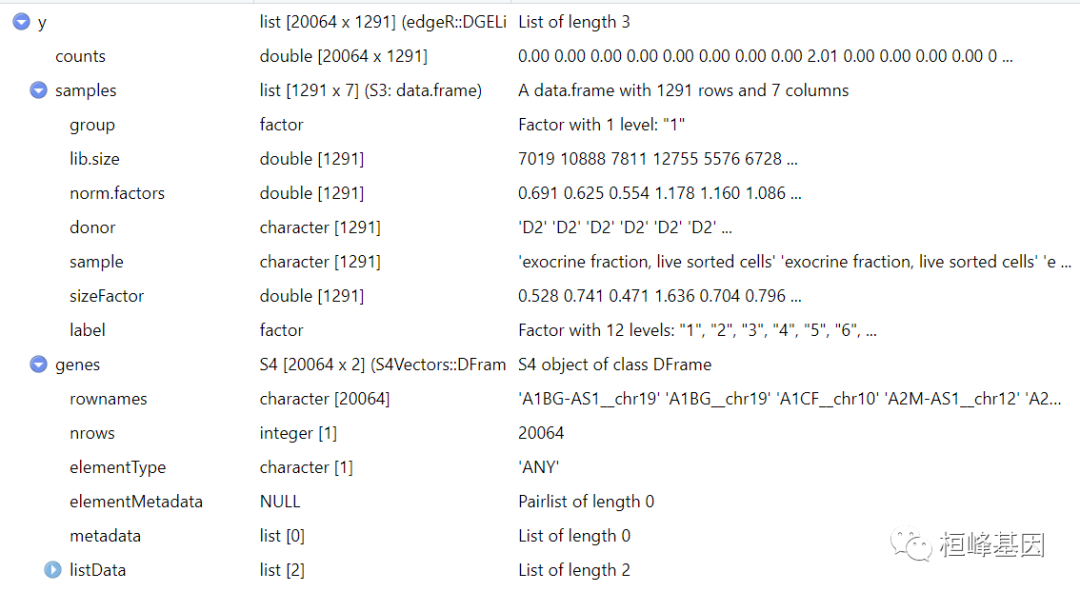
Reference
Grun, D., M. J. Muraro, J. C. Boisset, K. Wiebrands, A. Lyubimova, G. Dharmadhikari, M. van den Born, et al. 2016. “De Novo Prediction of Stem Cell Identity using Single-Cell Transcriptome Data.” Cell Stem Cell 19 (2): 266–77.
Lun, A. T., K. Bach, and J. C. Marioni. 2016. “Pooling across cells to normalize single-cell RNA sequencing data with many zero counts.” Genome Biol. 17 (April): 75.
Lun, A. T., D. J. McCarthy, and J. C. Marioni. 2016. “A step-by-step workflow for low-level analysis of single-cell RNA-seq data with Bioconductor.” F1000Res 5: 2122.
Xu, C., and Z. Su. 2015. “Identification of cell types from single-cell transcriptomes using a novel clustering method.” Bioinformatics 31 (12): 1974–80.
桓峰基因,铸造成功的您!
未来桓峰基因公众号将不间断的推出单细胞系列生信分析教程,
敬请期待!!
桓峰基因官网正式上线,请大家多多关注,还有很多不足之处,大家多多指正!
http://www.kyohogene.com/
桓峰基因和投必得合作,文章润色优惠85折,需要文章润色的老师可以直接到网站输入领取桓峰基因专属优惠券码:KYOHOGENE,然后上传,付款时选择桓峰基因优惠券即可享受85折优惠哦!https://www.topeditsci.com/