基于MPC的自适应巡航控制（Matlab代码实现）

news2025/10/30 2:02:09

💥💥💞💞欢迎来到本博客❤️❤️💥💥

🏆博主优势：🌞🌞🌞博客内容尽量做到思维缜密，逻辑清晰，为了方便读者。

⛳️座右铭：行百里者，半于九十。

📋📋📋本文目录如下：🎁🎁🎁

目录

💥1 概述

📚2 运行结果

🎉3 参考文献

🌈4 Matlab代码实现

💥1 概述

自适应巡航控制 (ACC) 系统又称主动巡航控制系统, 是在传统定速巡航控制基础上结合了车距保持功能, 利用车载雷达探测前方行驶环境, 通过控制节气门和制动系统自动调整车速, 提高驾驶舒适性和安全性.

ACC的历史可以追溯至20世纪70年代, 1971年, 美国EATON (伊顿) 公司便已从事这方面的开发, 其雏形是日本三菱公司提出的PDC (preview distance control) 系统.1995年三菱汽车在日本市场推出首款ACC系统, 此后丰田、本田、通用、福特、戴姆勒、博世等公司也投入研发行列.纵观ACC系统的发展历程, 可以分为三个阶段:第一阶段为20世纪90年代初针对高速公

路的ACC系统, 主要实现定速巡航和安全车距功能;第二阶段为20世纪90年代末针对城市工况的ACC系统, 即起-停巡航系统 (stop&go cruise control, SG-ACC) , 实现自动起步、停车和低速跟车功能;第三阶段为21世纪初至今综合考虑燃油经济性、跟踪性能和驾驶员感受的多目标协调式ACC系统.此外, ACC的功能也在不断扩展,如将ACC与车道保持相结合、ACC与避撞相结合、ACC与车道变更相结合等, 突破传统ACC仅纵向跟车功能局限, 进一步实现汽车辅助安全驾驶.

本文基于预测控制模型的自适应巡航控制仿真与机器人实现：

在两辆车之间已经达到了近乎精确的纵向模型
试图使控制响应接近可行性和真实条件。
满足防撞和保持安全距离，前车为主要目标，舒适性为次要目标。（控制应用于以下汽车）
在 MATLAB 上应用实现和仿真。

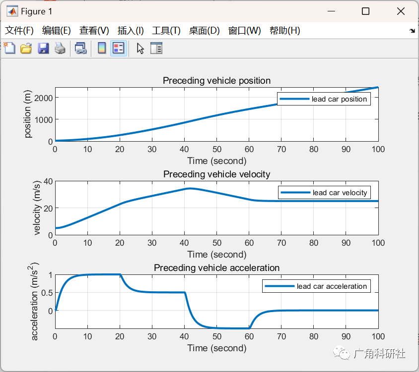
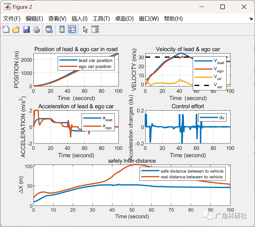
📚2 运行结果

主函数部分代码：

clear ;
close all;
clc

% Define the sample time, |Ts|, and simulation duration, |t|, in seconds.
t0 = 0;
Ts = 0.1;
Tf = 100;
t = t0:Ts:Tf;               
Nt = numel(t);
% Specify the initial position and velocity for the two vehicles.

%x0_lead = 0;               %Initial position of lead car (m)
%v0_lead = 0;               %Initial velocity of lead car (m/s)

%x0_ego = 0;                %Initial position of ego car (m)
%v0_ego = 0;                %Initial velocity of ego car (m/s)

% The safe distance between the lead car and the ego car is a function
% of the ego car velocity, $V_{ego}$:
%
% $$ D_{safe} = D_{default} + T_{gap}\times V_{ego} $$
%
% where $D_{default}$ is the standstill default spacing and $T_{gap}$ is
% the time gap between the vehicles. Specify values for $D_{default}$, in
% meters, and $T_{gap}$, in seconds.
t_gap = 1.4;
D_default = 10;

% Specify the driver-set velocity in m/s.
v_set = 30;

% Considering the physical limitations of the vehicle dynamics, the
% acceleration is constrained to the range  |[-3,2]| (m/s^2).
a_max = 2; da_max = 0.15;
a_min = -3; da_min = -0.2;



% the relationship between the actual acceleration and the desired 
% acceleration of the host vehicle satisfies the following conditions 
% 
%  $$ a(k+1) = (1-\frac{Ts}{\tau}) \times a(k) + \frac{Ts}{\tau} \times u(k)$$
%  
% where $ \tau $ is the time lag of the ACC system
tau = 0.3;


%Np = 20 ;          % Prediction Horizon
%Nc = 20 ;          % Control Horizon

%% Examples
%  In this section we want to try to specify the various parameters 
%   of the machine for different simulation


%EX.1
% N = 5;
% Np = 20 ;          % Prediction Horizon
% Nc = 5 ;          % Control Horizon
% x0_ego  = 0;
% v0_ego  = 0;
% x0_lead = 50;
% v0_lead = 15;
% a_lead = 0.3*sin(2*pi*0.03*t);  % Acceleration of lead car is a disturbance for our plant;
% [lead_car_position , lead_car_velocity] = lead_car_simulation(x0_lead,v0_lead,a_lead,t,Ts ,tau);

% EX.2
N = 5;
Np = 20 ;          % Prediction Horizon
Nc = 15 ;          % Control Horizon
x0_ego  = 0;
v0_ego  = 0;
x0_lead = 20;
v0_lead = 5;
a_lead = [1*(1-exp(-0.5*t(1:floor(Nt/5)))) ,0.5+0.5*exp(-0.5*t(1:floor(Nt/5))) , -0.5+exp(-0.5*t(1:floor(Nt/5))) ,-0.5*exp(-0.5*t(1:floor(Nt/5))) , zeros(1,floor(Nt/5)+1)];  
[lead_car_position , lead_car_velocity] = lead_car_simulation(x0_lead,v0_lead,a_lead,t,Ts ,tau);

% % % EX.3
% Np = 20 ;          % Prediction Horizon
% Nc = 15 ;          % Control Horizon
% x0_ego  = 0;
% v0_ego  = 0;
% x0_lead = 1500;
% v0_lead = 0;
% a_lead = zeros(1,Nt) ;
% [lead_car_position , lead_car_velocity] = lead_car_simulation(x0_lead,v0_lead,a_lead,t,Ts ,tau);

%% Car State Space Model

Am=[1   Ts   0.5*Ts^2
    0   1      Ts
    0   0     1-Ts/tau ];

Bm=[0 ; 0 ; Ts/tau];

Cm=[1   0  0
    0   1  0];


n = size(Am , 1) ;  % number of eigenvalues
q = size(Cm , 1) ;  % number of outputs
m = size(Bm , 2) ;  % number of inputs


[A , B , C] = AugemenFun(Am , Bm , Cm) ;

a = 0.5 ;
[Al , L0] = LagFun(N,a);
L = zeros( N , Nc ); 
L( : , 1) = L0 ; 
for i = 2:Nc
    L(:,i) = Al*L(: , i-1) ; 
end