博主前期相关的博客可见下：
机器学习项目实战-能源利用率 Part-1（数据清洗）
机器学习项目实战-能源利用率 Part-2（探索性数据分析）
机器学习项目实战-能源利用率 Part-3（特征工程与特征筛选）
机器学习项目实战-能源利用率 Part-4（模型构建）
这部分进行的是：模型解释。

导入建模数据

# import warning
# warning.filterwarning('ignore')

import pandas as pd
import numpy as np
pd.options.mode.chained_assignment = None
pd.set_option('display.max_columns', 50)

import matplotlib.pyplot as plt
import seaborn as sns
%matplotlib inline
plt.rcParams['font.size'] = 24
sns.set(font_scale = 2)

train_features = pd.read_csv('data/training_features.csv')
test_features = pd.read_csv('data/testing_features.csv')
train_labels = pd.read_csv('data/training_labels.csv')
test_labels = pd.read_csv('data/testing_labels.csv')

from sklearn.impute import SimpleImputer
imputer = SimpleImputer(strategy = 'median')
imputer.fit(train_features)
X = imputer.transform(train_features)
X_test = imputer.transform(test_features)

from sklearn.preprocessing import MinMaxScaler
minmax_scaler = MinMaxScaler().fit(X)
X = minmax_scaler.transform(X)
X_test = minmax_scaler.transform(X_test)

y = np.array(train_labels).reshape((-1, ))
y_test = np.array(test_labels).reshape((-1, ))

def mae(y_true, y_pred):
	return np.mean(abs(y_true - y_pred))

from sklearn.ensemble import GradientBoostingRegressor

model = GradientBoostingRegressor(loss = 'lad', max_depth = 6, max_features = None,
                                 min_samples_leaf = 4, min_samples_split = 10, n_estimators = 550, random_state = 42)
model.fit(X, y)

model_pred = model.predict(X_test)
model_mae = mae(y_test, model_pred)
print('Final Model Performance on the test set: MAE = %.4f' % model_mae)

这段代码用于构建一个梯度提升回归模型，并在测试数据集上评估其性能。

• import pandas as pd、import numpy as np、pd.options.mode.chained_assignment = None、pd.set_option('display.max_columns', 50)、import matplotlib.pyplot as plt、import seaborn as sns和%matplotlib inline：导入所需的Python库，并设置显示选项。
• plt.rcParams['font.size'] = 24和sns.set(font_scale = 2)：设置字体大小和缩放比例。
• from sklearn.impute import SimpleImputer和imputer = SimpleImputer(strategy = 'median')：从sklearn.impute模块中导入SimpleImputer类，用于填补缺失值。创建一个SimpleImputer对象imputer，使用中位数策略来填补缺失值，即将每个特征的缺失值替换为该特征的中位数。
• imputer.fit(train_features)：使用训练特征数据集train_features来拟合imputer对象，计算每个特征的中位数。
• X = imputer.transform(train_features)和X_test = imputer.transform(test_features)：使用imputer对象对训练特征数据集train_features和测试特征数据集test_features进行缺失值填补，分别将填补后的特征数据存储在名为X和X_test的NumPy数组中。
• from sklearn.preprocessing import MinMaxScaler和minmax_scaler = MinMaxScaler().fit(X)：从sklearn.preprocessing模块中导入MinMaxScaler类，用于将特征数据进行标准化。创建一个MinMaxScaler对象minmax_scaler并使用训练特征数据集X来拟合minmax_scaler对象，计算每个特征的最小值和最大值。
• X = minmax_scaler.transform(X)和X_test = minmax_scaler.transform(X_test)：使用minmax_scaler对象对训练特征数据集X和测试特征数据集X_test进行标准化处理，分别将标准化后的特征数据存储在名为X和X_test的NumPy数组中。
• y = np.array(train_labels).reshape((-1, ))和y_test = np.array(test_labels).reshape((-1, ))：将训练标签数据集train_labels和测试标签数据集test_labels转换为NumPy数组，并将它们展平为一维数组，分别存储在名为y和y_test的变量中。
• def mae(y_true, y_pred): return np.mean(abs(y_true - y_pred))：定义一个计算平均绝对误差（MAE）的函数mae，其中y_true表示真实标签，y_pred表示预测标签。
• from sklearn.ensemble import GradientBoostingRegressor和model = GradientBoostingRegressor(loss = 'lad', max_depth = 6, max_features = None, min_samples_leaf = 4, min_samples_split = 10, n_estimators = 550, random_state = 42)：从sklearn.ensemble模块中导入GradientBoostingRegressor类，用于构建梯度提升回归模型。创建一个GradientBoostingRegressor对象model，并使用指定的参数对模型进行初始化，包括损失函数为lad（最小绝对误差），最大树深度为6，最大特征数为None（即使用所有特征），最小叶节点样本数为4，最小分裂节点样本数为10，估计器的数量为550，随机种子为42。
• model.fit(X, y)：使用训练特征数据集X和训练标签数据集y来拟合model对象，训练梯度提升回归模型。
• model_pred = model.predict(X_test)：使用测试特征数据集X_test来进行预测，生成预测结果，存储在名为model_pred的变量中。
• model_mae = mae(y_test, model_pred)：使用测试标签数据集y_test和模型预测的结果model_pred来计算模型的MAE，将结果存储在名为model_mae的变量中。
• print('Final Model Performance on the test set: MAE = %.4f' % model_mae)：将模型在测试数据集上的MAE输出到控制台。

模型解释

从下面三个方面进行解释：

• 特征重要性
• Locally Interpretable Model-agnostic Explainer (LIME)
• 建立一颗树模

特征重要性

在所有树模型中平均节点不纯度的减少

特征重要性排序

feature_results = pd.DataFrame({'feature': list(train_features.columns),
                               'importance': model.feature_importances_})
feature_results = feature_results.sort_values('importance', ascending = False).reset_index(drop = True)
feature_results.head(8)

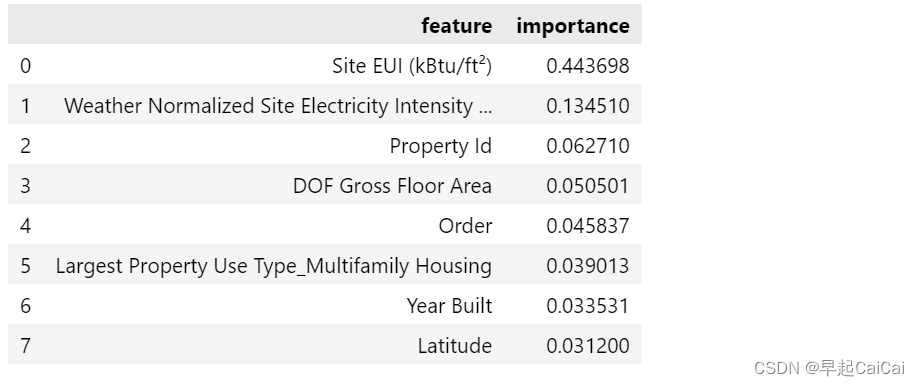
这段代码用于计算并输出梯度提升回归模型中每个特征的重要性分数，以及显示具有最高重要性分数的前8个特征。

• feature_results = pd.DataFrame({'feature': list(train_features.columns), 'importance': model.feature_importances_})：创建一个名为feature_results的数据框，其中包含两列：feature和importance。feature列包含训练特征数据集中的所有特征的名称，使用list(train_features.columns)来获取特征名称列表；importance列包含每个特征的重要性分数，使用model.feature_importances_来获取模型的特征重要性分数。
• feature_results = feature_results.sort_values('importance', ascending = False).reset_index(drop = True)：按照特征的重要性分数对feature_results数据框进行降序排序，即从高到低排序。'importance'表示按照重要性分数进行排序，ascending=False表示降序排列。排序后使用reset_index函数将索引重置为默认值，并将drop参数设置为True以删除旧索引列，将排序后的结果存储回feature_results数据框中。
• feature_results.head(8)：输出具有最高重要性分数的前8个特征。使用head函数选择前8行，这里的8是作为函数的参数传递进去的，因此可以自定义显示的行数，这里是选择前8行。

from IPython.core.pylabtools import figsize
figsize(12, 10)
plt.style.use('ggplot')

feature_results.loc[:9, :].plot(x = 'feature', y = 'importance', edgecolor = 'k',
                               kind = 'barh', color = 'blue')
plt.xlabel('Relative Importance', fontsize = 18); plt.ylabel('')
# plt.yticks(fontsize = 12); plt.xticks(fontsize = 14)
plt.title('Feature Importances from Random Forest', size = 26)

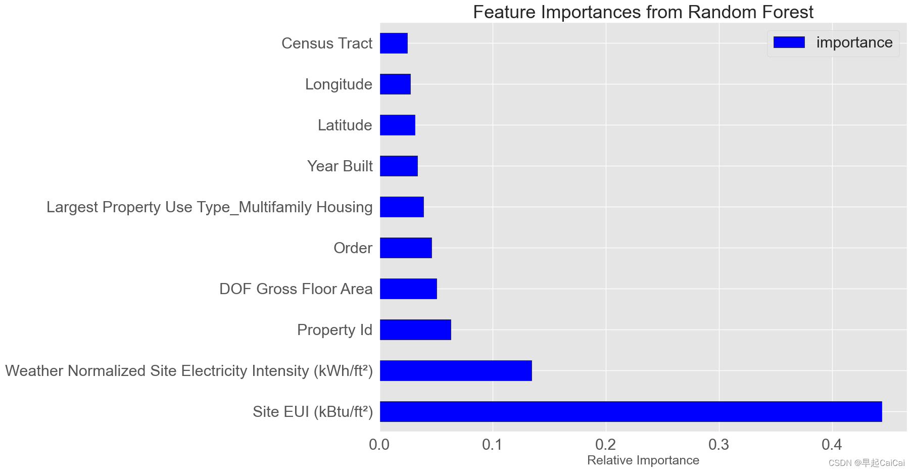
上图是将特征重要性绘制成图

cumulative_importances = np.cumsum(feature_results['importance'])

plt.figure(figsize = (20, 6))
plt.plot(list(range(feature_results.shape[0])), cumulative_importances.values, 'b-')
plt.hlines(y=0.95, xmin=0, xmax=feature_results.shape[0], color='r', linestyles='dashed')
# plt.xticks(list(range(feature_results.shape[0])), feature_results.feature, rotation=60)
plt.xlabel('Feature', fontsize = 18)
plt.ylabel('Cumulative importance', fontsize = 18)
plt.title('Cumulative Importances', fontsize = 26)

这段代码用于绘制累积特征重要性曲线图，以展示所有特征对目标变量的总贡献度，并标记出贡献度达到95%的阈值。

• cumulative_importances = np.cumsum(feature_results['importance'])：计算每个特征对目标变量的重要性分数的累积总和，使用np.cumsum函数将特征重要性分数进行累加，将结果存储在名为cumulative_importances的变量中。
• plt.figure(figsize = (20, 6))：创建一个名为figure的图形对象，大小为20英寸×6英寸。
• plt.plot(list(range(feature_results.shape[0])), cumulative_importances.values, 'b-')：绘制累积特征重要性曲线，使用plt.plot函数绘制，横坐标是特征的序号，纵坐标是特征的重要性分数的累积总和，颜色为蓝色，线型为实线。
• plt.hlines(y=0.95, xmin=0, xmax=feature_results.shape[0], color='r', linestyles='dashed')：在y=0.95处绘制一条水平线，表示累积重要性分数达到95%的阈值。使用plt.hlines函数绘制水平线，y=0.95表示水平线的高度，xmin=0表示x轴的起点，xmax=feature_results.shape[0]表示x轴的终点，即特征的个数。颜色为红色，线型为虚线。
• plt.xlabel('Feature', fontsize = 18)、plt.ylabel('Cumulative importance', fontsize = 18)和plt.title('Cumulative Importances', fontsize = 26)：设置x轴标签为“Feature”，y轴标签为“Cumulative importance”，图形标题为“Cumulative Importances”，并分别设置它们的字体大小为18和26。

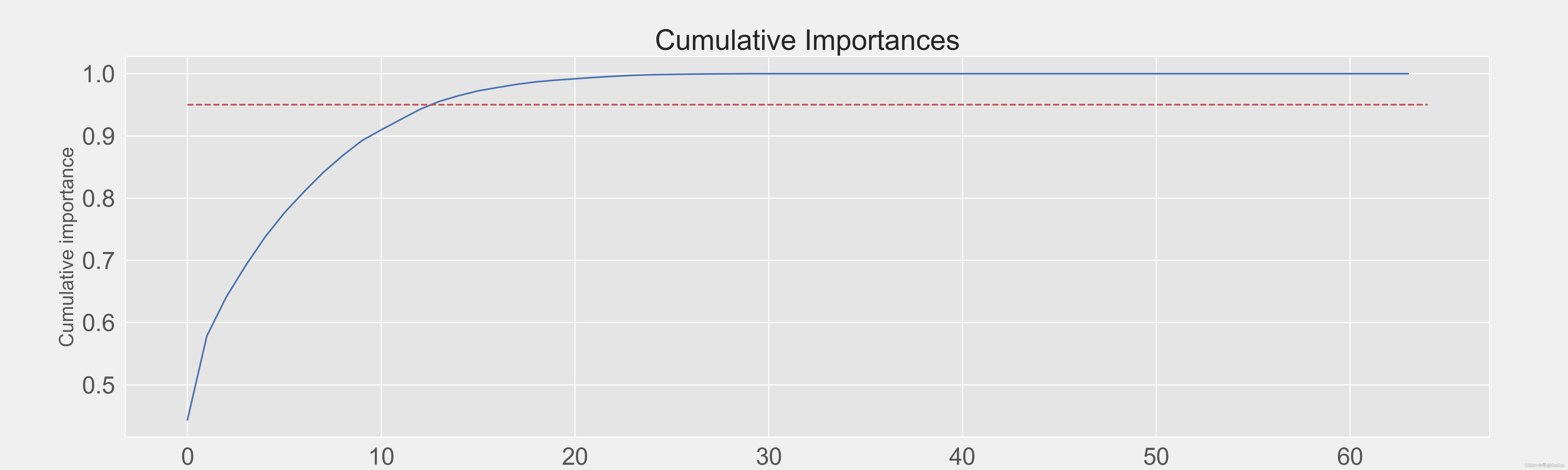
most_num_importances = np.where(cumulative_importances > 0.95)[0][0] + 1
print('Number of features for 95% importance: ', most_num_importances)

累计的特征超过0.95

根据特征重要性筛选特征

most_important_features = feature_results['feature'][:13]
indices = [list(train_features.columns).index(x) for x in most_important_features]
X_reduced = X[:, indices]
X_test_reduced = X_test[:, indices]

print('Most import training features shape: ', X_reduced.shape)
print('Most import testing feature shape: ', X_test_reduced.shape)

根据特征重要性筛选特征

from sklearn.ensemble import RandomForestRegressor
rfr = RandomForestRegressor(random_state = 42)

rfr.fit(X, y)
rfr_full_pred = rfr.predict(X_test)

rfr.fit(X_reduced, y)
rfr_reduced_pred = rfr.predict(X_test_reduced)

print('Random Forest Full Results: MAE =    %.4f.' % mae(y_test, rfr_full_pred))
print('Random Forest Reduced Results: MAE = %.4f.' % mae(y_test, rfr_reduced_pred))

from sklearn.linear_model import LinearRegression
lr = LinearRegression()

lr.fit(X, y)
lr_full_pred = lr.predict(X_test)

lr.fit(X_reduced, y)
lr_reduced_pred = lr.predict(X_test_reduced)

print('Linear Regression Full Results: MAE =    %.4f.' % mae(y_test, lr_full_pred))
print('Linear Regression Reduced Results: MAE = %.4f.' % mae(y_test, lr_reduced_pred))

这段代码用于比较使用完整特征集和精简特征集分别训练的随机森林回归模型和线性回归模型在测试数据集上的性能差异。

• from sklearn.ensemble import RandomForestRegressor和rfr = RandomForestRegressor(random_state = 42)：从sklearn.ensemble模块中导入RandomForestRegressor类，用于构建随机森林回归模型。创建一个RandomForestRegressor对象rfr，并使用指定的参数对模型进行初始化，包括随机种子为42。
• rfr.fit(X, y)和rfr_full_pred = rfr.predict(X_test)：使用完整特征集X和训练标签数据集y来拟合rfr对象，训练随机森林回归模型。使用测试特征数据集X_test进行预测，生成预测结果，存储在名为rfr_full_pred的变量中。
• rfr.fit(X_reduced, y)和rfr_reduced_pred = rfr.predict(X_test_reduced)：使用精简特征集X_reduced和训练标签数据集y来拟合rfr对象，训练随机森林回归模型。使用精简特征集X_test_reduced进行预测，生成预测结果，存储在名为rfr_reduced_pred的变量中。
• print('Random Forest Full Results: MAE = %.4f.' % mae(y_test, rfr_full_pred))和print('Random Forest Reduced Results: MAE = %.4f.' % mae(y_test, rfr_reduced_pred))：分别打印输出随机森林回归模型在测试数据集上的MAE（平均绝对误差）评估结果。第一行输出使用完整特征集训练的模型的评估结果，第二行输出使用精简特征集训练的模型的评估结果。mae函数用于计算预测结果和真实标签的MAE值。
• from sklearn.linear_model import LinearRegression和lr = LinearRegression()：从sklearn.linear_model模块中导入LinearRegression类，用于构建线性回归模型。创建一个LinearRegression对象lr，用于训练线性回归模型。
• lr.fit(X, y)和lr_full_pred = lr.predict(X_test)：使用完整特征集X和训练标签数据集y来拟合lr对象，训练线性回归模型。使用测试特征数据集X_test进行预测，生成预测结果，存储在名为lr_full_pred的变量中。
• lr.fit(X_reduced, y)和lr_reduced_pred = lr.predict(X_test_reduced)：使用精简特征集X_reduced和训练标签数据集y来拟合lr对象，训练线性回归模型。使用精简特征集X_test_reduced进行预测，生成预测结果，存储在名为lr_reduced_pred的变量中。
• print('Linear Regression Full Results: MAE = %.4f.' % mae(y_test, lr_full_pred))和print('Linear Regression Reduced Results: MAE = %.4f.' %mae(y_test, lr_reduced_pred))：分别打印输出线性回归模型在测试数据集上的MAE（平均绝对误差）评估结果。第一行输出使用完整特征集训练的模型的评估结果，第二行输出使用精简特征集训练的模型的评估结果。mae函数用于计算预测结果和真实标签的MAE值。
  

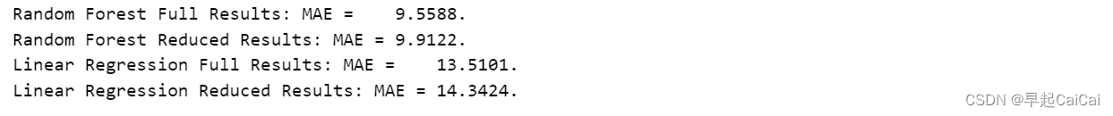
试验结果发现效果还不如原来
但仅考虑更少的特征就能得到一个还不错的效果

model_reduced = GradientBoostingRegressor(loss = 'lad', max_depth = 6, max_features = None,
                                 min_samples_leaf = 4, min_samples_split = 10,
                                 n_estimators = 550, random_state = 42)
model_reduced.fit(X_reduced, y)
model_reduced_pred = model_reduced.predict(X_test_reduced)

print('Gradient Boosting Reduced Results: MAE = %.4f.' % mae(y_test, model_reduced_pred))

在这里是9.48；之前的case是9.12
更多的特征会得到更好的效果

LIME

Locally Interpretable Model-agnostic Explanations

“局部可解释的模型无关解释”，简称LIME。它是一种用于解释机器学习模型预测的方法，可以在不需要了解模型内部结构的情况下，对模型的预测结果进行可解释的解释。
GitHub - LIME to explain individual predictions

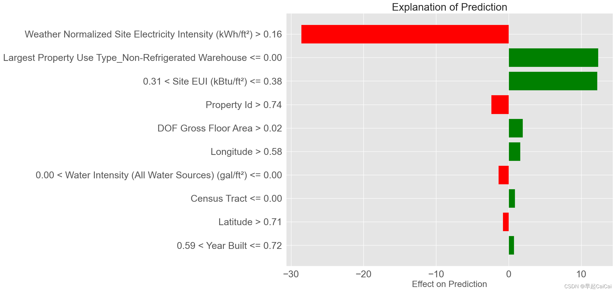
最差预测的解释

import lime
import lime.lime_tabular

residuals = abs(model_reduced_pred - y_test) # 残差
wrong = X_test_reduced[np.argmax(residuals), :] # 最差的预测
right = X_test_reduced[np.argmin(residuals), :] # 最好的预测

# 最差预测位置的预测值与真实值
print('Prediction: %.4f' % model_reduced.predict(wrong.reshape(1, -1)))
print('Actual Value: %.4f' % y_test[np.argmax(residuals)])

# Create a lime explainer object
explainer = lime.lime_tabular.LimeTabularExplainer(training_data = X_reduced, mode = 'regression',
            training_labels = y, feature_names = list(most_important_features))

# 最差预测的解释
wrong_exp = explainer.explain_instance(data_row = wrong, predict_fn = model_reduced.predict)

# 预测的解释画图
wrong_exp.as_pyplot_figure()
plt.title('Explanation of Prediction', fontsize = 24)
plt.xlabel('Effect on Prediction', fontsize = 20)

这段代码用于使用LIME（局部可解释的模型无关解释）对机器学习模型中最糟糕的预测进行解释，并生成一个解释图。

• import lime和import lime.lime_tabular：导入lime和lime.lime_tabular模块，用于构建和解释LIME模型。
• residuals = abs(model_reduced_pred - y_test)：计算机器学习模型在测试集上的预测残差，即预测值与真实值之间的差值的绝对值，使用abs函数计算。将结果存储在名为residuals的变量中。
• wrong = X_test_reduced[np.argmax(residuals), :]和right = X_test_reduced[np.argmin(residuals), :]：分别找到机器学习模型中预测残差最大和最小的测试样本。使用np.argmax和np.argmin函数找到残差数组residuals中最大值和最小值的索引，然后使用索引在测试特征数据集X_test_reduced中找到对应的样本特征，将最差的预测存储在名为wrong的变量中，将最好的预测存储在名为right的变量中。
• print('Prediction: %.4f' % model_reduced.predict(wrong.reshape(1, -1)))和print('Actual Value: %.4f' % y_test[np.argmax(residuals)])：分别打印输出最差预测位置的预测值和真实值。使用model_reduced.predict方法对wrong进行预测，将预测结果输出到屏幕上，使用y_test数组中最差预测的索引输出真实值。如果模型预测值与真实值相差很大，则该预测可能是错误的。
• explainer = lime.lime_tabular.LimeTabularExplainer(training_data = X_reduced, mode = 'regression', training_labels = y, feature_names = list(most_important_features))：创建一个LIME解释器对象explainer。使用lime.lime_tabular.LimeTabularExplainer类构建解释器，指定训练数据集X_reduced、训练标签数据集y、特征名称列表most_important_features和模型类型mode = 'regression'。这里使用的是基于表格数据的LIME解释器。
• wrong_exp = explainer.explain_instance(data_row = wrong, predict_fn = model_reduced.predict)：使用LIME解释器对象explainer对最差的预测进行解释。使用explain_instance方法对wrong进行解释，并将预测函数model_reduced.predict传递给predict_fn参数，以便LIME解释器可以近似原始模型的预测结果，并生成一个解释对象wrong_exp。
• wrong_exp.as_pyplot_figure()和plt.title('Explanation of Prediction', fontsize = 24)：将解释对象wrong_exp转换为Matplotlib图形对象，并显示在屏幕上。使用as_pyplot_figure方法将LIME解释器对象wrong_exp转换为Matplotlib图形对象，并使用plt.title方法设置图形标题为“Explanation of Prediction”，字体大小为24。

wrong_exp.show_in_notebook(show_predicted_value = False)

这段代码用于在Jupyter Notebook中显示最差预测的LIME解释图，并隐藏预测值。

• wrong_exp.show_in_notebook(show_predicted_value = False)：将最差预测的LIME解释图显示在Jupyter Notebook中，并将预测值隐藏。使用show_in_notebook方法将LIME解释对象wrong_exp显示为一个可交互的解释图。该方法有一个名为show_predicted_value的参数，用于控制是否在图形中显示预测值。这里将该参数设置为False，以隐藏预测值。

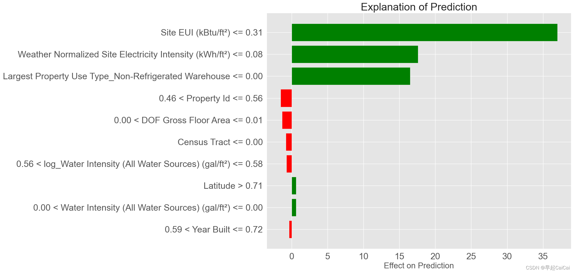
最好预测的解释

# 最好预测位置的预测值与真实值
print('Prediction: %0.4f' % model_reduced.predict(right.reshape(1, -1)))
print('Actual Value: %0.4f' % y_test[np.argmin(residuals)])

# 最好预测的解释
right_exp = explainer.explain_instance(data_row = right, predict_fn = model_reduced.predict, num_features = 10)

# 预测的解释画图
right_exp.as_pyplot_figure()
plt.title('Explanation of Prediction', size = 26)
plt.xlabel('Effect on Prediction', size = 20)

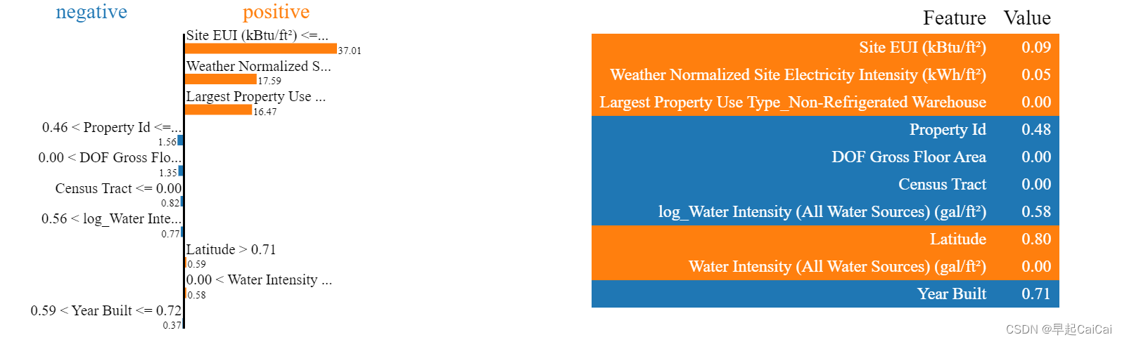
right_exp.show_in_notebook(show_predicted_value = False)

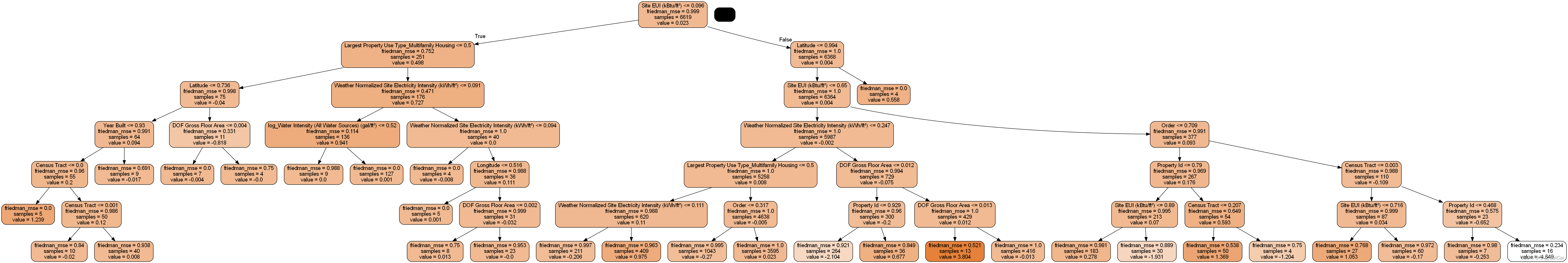
单棵树模型观察

from sklearn import tree
import pydotplus
from IPython.display import display, Image

single_tree = model_reduced.estimators_[100][0]

dot_data = tree.export_graphviz(single_tree, out_file = None, rounded = True,
                    feature_names = most_important_features, filled = True)
graph = pydotplus.graph_from_dot_data(dot_data)
graph.write_png('sigle_tree_1.png')

这段代码用于将随机森林模型中的单个决策树可视化为一张图。

• from sklearn import tree和import pydotplus：导入sklearn中的tree模块和pydotplus模块，用于可视化决策树。
• from IPython.display import display, Image：从IPython.display模块中导入display和Image函数，用于在Jupyter Notebook中显示图像。
• single_tree = model_reduced.estimators_[100][0]：从随机森林模型中提取第100个决策树，并将其存储在名为single_tree的变量中。model_reduced是随机森林模型对象，estimators_属性包含了随机森林中所有的决策树。
• dot_data = tree.export_graphviz(single_tree, out_file = None, rounded = True, feature_names = most_important_features, filled = True)：将单个决策树转换为Graphviz格式的数据，并将其存储在名为dot_data的变量中。使用tree.export_graphviz函数将single_tree转换为Graphviz格式的数据，设置out_file参数为None，以便将数据存储在内存中，设置rounded参数为True，以便在输出的节点框中使用圆角，设置feature_names参数为most_important_features，以便在决策树中使用特征名称，设置filled参数为True，以便在输出的节点框中使用填充色。
• graph = pydotplus.graph_from_dot_data(dot_data)：将Graphviz格式的数据转换为pydotplus中的图形对象，并将其存储在名为graph的变量中。使用pydotplus.graph_from_dot_data方法将dot_data转换为pydotplus中的图形对象，该对象可以用于生成PNG或PDF格式的图像。
• graph.write_png('sigle_tree_1.png')：将单个决策树的图像保存为PNG格式的文件。使用write_png方法将graph对象保存为PNG格式的图像文件，并将文件名设置为sigle_tree_1.png。

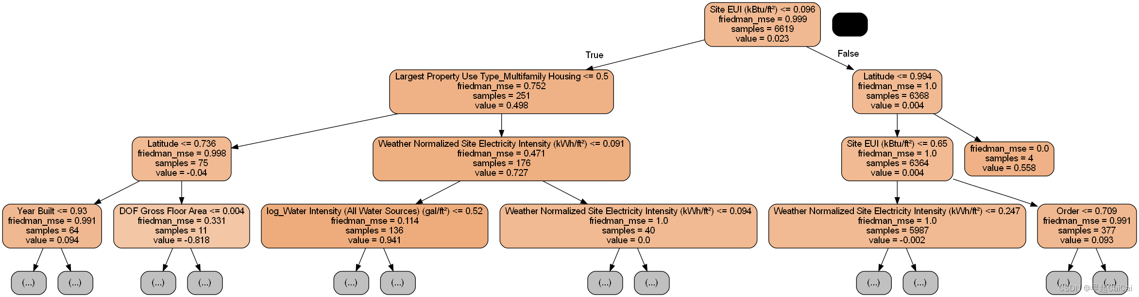
太密集了，限制下深度

dot_data = tree.export_graphviz(single_tree, out_file = None, rounded = True,
                    max_depth = 3, feature_names = most_important_features, filled = True)
graph = pydotplus.graph_from_dot_data(dot_data)
graph.write_png('sigle_tree_2.png')

End

Reference

机器学习项目实战-能源利用率 Part-1（数据清洗）

机器学习项目实战-能源利用率 Part-2（探索性数据分析）

机器学习项目实战-能源利用率 Part-3（特征工程与特征筛选）

机器学习项目实战-能源利用率 Part-4（模型构建）

机器学习项目实战-能源利用率3-分析