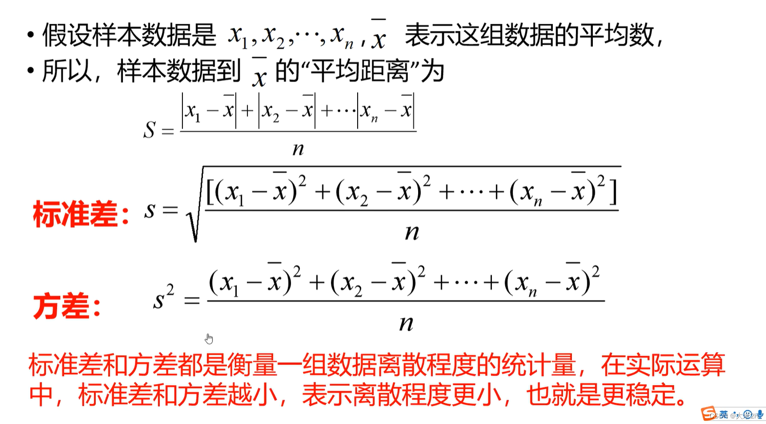
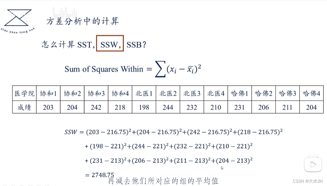
- 在分析数据之前,我们需要剔除异常值的影响,也就是在某个分组情况下,标准差过大(标准差越大,证明情况越不稳定),如果标准差比较小,就算是最小值和最大值差的比较大,我也认为他是一个比较平稳的波动。
- 方差分析这个老师讲的很好:[https://www.bilibili.com/video/BV1jB4y1676T/?spm_id_from=333.788&vd_source=642d9a85cff4a726a7de10f2383987df]
Step 6:Reduce Std.
- assure data stability
# 按 Category 列分组并计算每个分组的标准差
grouped_data = df_replen.groupby(['mot','country','priority','cc']).agg({'lt_pu_pod':['std','count',lambda x:x.quantile(0.9),lambda x:x.quantile(0.1)]})
# 打印结果
grouped_data = grouped_data.reset_index()
grouped_data.columns = ['mot','country','priority','cc','std','count','quantile_90','quantile_10']
grouped_data
| mot | country | priority | cc | std | count | quantile_90 | quantile_10 | |
|---|---|---|---|---|---|---|---|---|
| 0 | SEA | AE | 40 | AD | NaN | 1 | 10.360 | 10.360 |
3150 rows × 8 columns
for group_i in grouped_data.index:
    group_mot = grouped_data.loc[group_i,'mot']
    group_country = grouped_data.loc[group_i,'country']
    group_priority = grouped_data.loc[group_i,'priority']
    group_cc = grouped_data.loc[group_i,'cc']

    group_std = grouped_data.loc[group_i,'std']
    group_count = grouped_data.loc[group_i,'count']
    group_quantile_90 = grouped_data.loc[group_i,'quantile_90']
    group_quantile_10 = grouped_data.loc[group_i,'quantile_10']

    if group_count>=5 and group_std>=8:
        index_replen = df_replen[(df_replen['mot']==group_mot) & (df_replen['country']==group_country) & (df_replen['priority']==group_priority)
                 & ((df_replen['lt_pu_pod']>=group_quantile_90) | (df_replen['lt_pu_pod']<=group_quantile_10))
                 ].index
        for repl_i in index_replen:
            df_replen.loc[repl_i,'Type_'] = 'Y'
df_replen_1 = df_replen[df_replen['Type_'].isnull()]
df_replen_1 = df_replen_1[~df_replen_1['hawb'].isnull() & ~df_replen_1['ts_atd'].isnull() & ~df_replen_1['cc'].isnull() & ~df_replen_1['weight'].isnull()].reset_index().drop('index',axis=1)
df_replen_1.info()
<class 'pandas.core.frame.DataFrame'>
RangeIndex: 103166 entries, 0 to 103165
Data columns (total 24 columns):
 #   Column             Non-Null Count   Dtype
---  ------             --------------   -----
 0   hawb               103233 non-null  object
 1   mot                103233 non-null  object
 2   geo                103166 non-null  object
 3   country            103166 non-null  object
 4   shippingfrequency  103166 non-null  object
 5   isgreen            103166 non-null  object
 6   priority           103166 non-null  object
 7   forwarder          103166 non-null  object
 8   cc                 93166 non-null  object
 9   dn_gr_status       103166 non-null  object
 10  volume             103166 non-null  float64
 11  weight             103166 non-null  float64
 12  dn_seq_qty         103166 non-null  float64
 13  ts_pu              103166 non-null  object
 14  ts_atd             103166 non-null  object
 15  ts_ata             103038 non-null  object
 16  ts_cc              102855 non-null  object
 17  ts_pod             103166 non-null  object
 18  ts_atd_pre_2_date  103166 non-null  object
 19  lt_pu_pod          103166 non-null  float64
 20  lt_pu_atd          103166 non-null  float64
 21  lt_atd_ata         103166 non-null  float64
 22  data_source        103166 non-null  object
 23  Type_              0 non-null       object
dtypes: float64(6), object(18)
memory usage: 18.9+ MB
# 按 Category 列分组并计算每个分组的标准差
grouped_data_1 = df_replen_1.groupby(['mot','country','priority','cc']).agg({'lt_pu_pod':['std','count',lambda x:x.quantile(0.9),lambda x:x.quantile(0.1)]})
# 打印结果
grouped_data_1 = grouped_data_1.reset_index()
grouped_data_1.columns = ['mot','country','priority','cc','std','count','quantile_90','quantile_10']
grouped_data_1
| mot | country | priority | cc | std | count | quantile_90 | quantile_10 | |
|---|---|---|---|---|---|---|---|---|
| 0 | AIR | ER | 30 | AD | NaN | 1 | 16.333 | 16.333 |
3017 rows × 8 columns
print('Reduce std','As is:【',grouped_data['std'].mean(),'-->','】To be:【',grouped_data_1['std'].mean(),'】')
Reduce std As is:【 4.281785006069334 --> 】To be:【 2.748443864082784 】
Step 7:Research Relationship
research weight&leadtime relationship
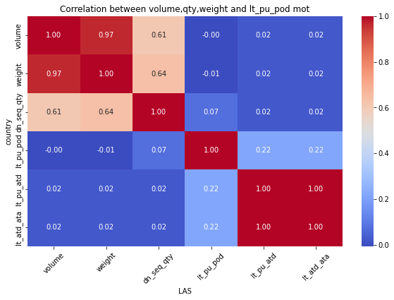
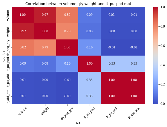
for mot in df_replen_1['geo'].unique().tolist():
    plt.figure(figsize=(10, 6))
    sns.heatmap(data=df_replen_1[(df_replen_1['geo']==mot)].corr(), cmap='coolwarm', annot=True, fmt=".2f", cbar=True)
    plt.title("Correlation between volume,qty,weight and lt_pu_pod mot")
    plt.xlabel("{0}".format(mot))
    plt.ylabel("country")
    plt.xticks(rotation=45)
    plt.show()
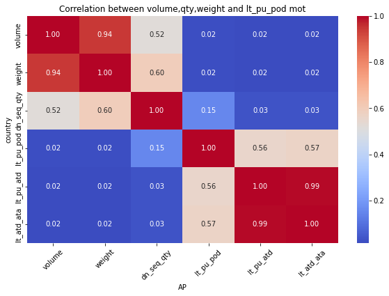
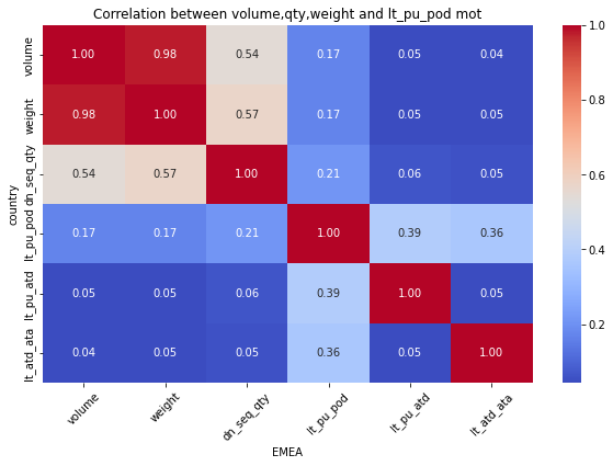
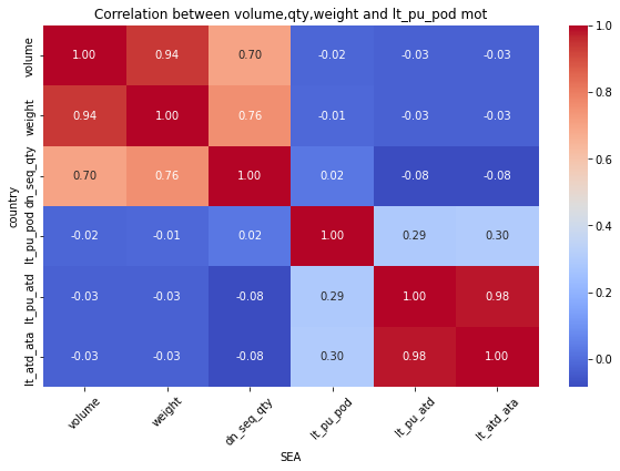
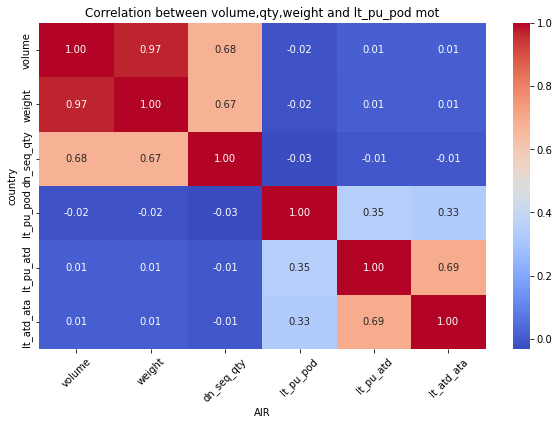
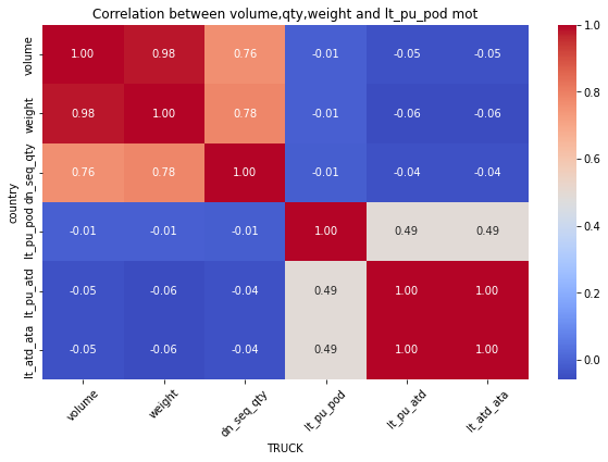
for mot in df_replen_1['mot'].unique().tolist():
    plt.figure(figsize=(10, 6))
    sns.heatmap(data=df_replen_1[(df_replen_1['mot']==mot)].corr(), cmap='coolwarm', annot=True, fmt=".2f", cbar=True)
    plt.title("Correlation between volume,qty,weight and lt_pu_pod mot")
    plt.xlabel("{0}".format(mot))
    plt.ylabel("country")
    plt.xticks(rotation=45)
    plt.show()
-
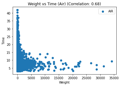
Consequently:weight&dn_seq_qty is Strong correlation relationship
-
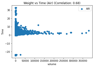
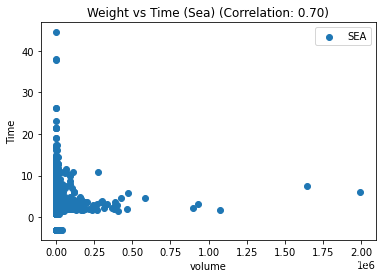
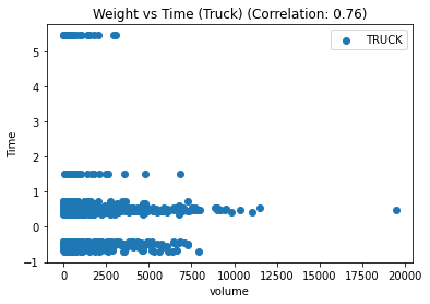
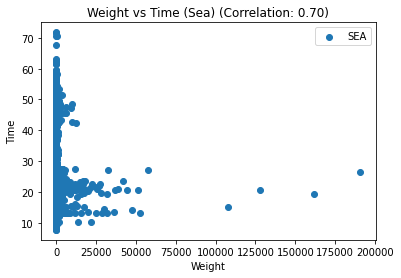
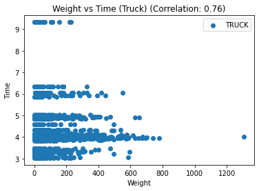
but weight&leadtime is weak correlation relationship
# 计算相关系数
corr = df_replen_1.corr().iloc[0,1]

# 按照运输类型分组并绘制散点图
for t, group in df_replen_1.groupby('mot'):
    plt.scatter(group['volume'], group['lt_pu_atd'], label=t)
    corr = group.corr().iloc[0,2]
    # 添加图标题和坐标轴标签
    plt.title(f"Weight vs Time ({t.title()}) (Correlation: {corr:.2f})")
    plt.xlabel("volume")
    plt.ylabel("Time")

    # 添加图例
    plt.legend()

    # 显示图形
    plt.show()
# 计算相关系数
corr = df_replen_1.corr().iloc[0,1]

# 按照运输类型分组并绘制散点图
for t, group in df_replen_1.groupby('mot'):
    plt.scatter(group['weight'], group['lt_pu_pod'], label=t)
    corr = group.corr().iloc[0,2]
    # 添加图标题和坐标轴标签
    plt.title(f"Weight vs Time ({t.title()}) (Correlation: {corr:.2f})")
    plt.xlabel("Weight")
    plt.ylabel("Time")

    # 添加图例
    plt.legend()

    # 显示图形
    plt.show()
方差1、GEO与LT_PU_POD的关联性

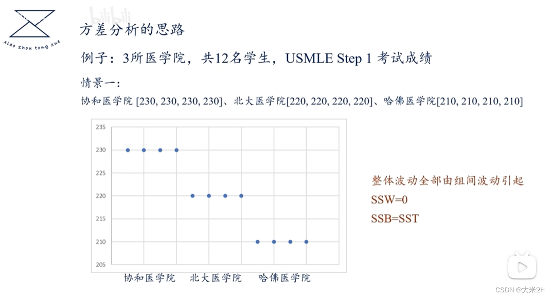
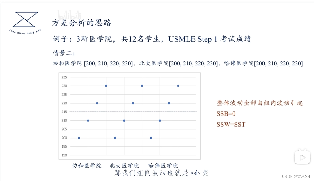


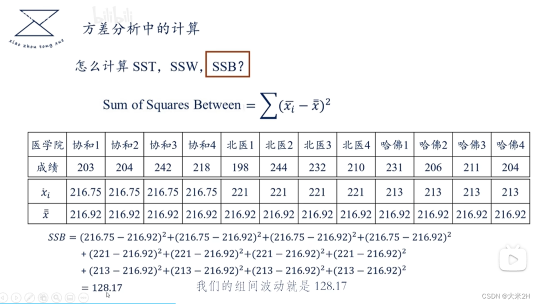

方差分析
- 原假设:每个GEO直接与LT_PU_POD没有关联性
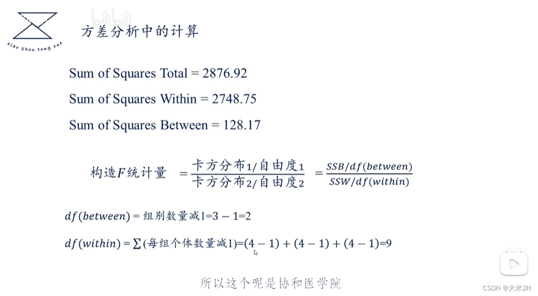
在独立样本T检验中,自由度的计算方法与样本数量有关。如果你有4个geo,假设每个geo对应一个独立的样本组别,那么自由度的计算如下:
自由度 = (样本1的观测数量 - 1) + (样本2的观测数量 - 1) + … + (样本4的观测数量 - 1)
具体计算时,需要知道每个geo对应的样本数量。假设分别为n1、n2、n3、n4,则自由度为 (n1 - 1) + (n2 - 1) + (n3 - 1) + (n4 - 1)。
df_replen_1.groupby(['geo']).agg({'lt_pu_pod':['std','count','mean',lambda x:x.quantile(0.5),lambda x:x.quantile(0.9),lambda x:x.quantile(0.1)]}).reset_index()
| geo | lt_pu_pod | ||||||
|---|---|---|---|---|---|---|---|
| std | count | mean | <lambda_0> | <lambda_1> | <lambda_2> | ||
| 0 | EA | 3.444 | 47424 | 8.940807 | 6.35 | 17.53 | 3.98 |
| 1 | Brazil | NaN | 1 | 7.830000 | 7.83 | 7.83 | 7.83 |
| 2 | MX | 8.325913 | 22476 | 7.995670 | 6.34 | 9.43 | 3.87 |
| 3 | NE | 7.462291 | 7542 | 15.752510 | 14.32 | 26.35 | 7.39 |
| 4 | PJ | 5.333 | 6861 | 9.633206 | 8.12 | 17.43 | 5.43 |
from scipy.stats import f_oneway

# 提取不同地理位置的运输耗时数据
geo1_data = df_replen_1[df_replen_1['geo'] == 'AP']['lt_pu_pod']
geo2_data = df_replen_1[df_replen_1['geo'] == 'EMEA']['lt_pu_pod']
geo3_data = df_replen_1[df_replen_1['geo'] == 'LAS']['lt_pu_pod']
geo4_data = df_replen_1[df_replen_1['geo'] == 'NA']['lt_pu_pod']

# 执行单因素方差分析
f_stat, p_value = f_oneway(geo1_data, geo2_data, geo3_data, geo4_data)

# 输出分析结果
print("单因素方差分析结果:")
print("F统计量:", f_stat)
print("p值:", p_value)
单因素方差分析结果:
F统计量: 2676.3050920291266
p值: 0.0
- 当p值等于0时,通常表示在检验中观察到的差异极其显著。这意味着在假设检验中,得到的样本数据非常不可能出现,或者可以说观察到的差异非常显著,远远超过了我们预期的随机差异。
方差2、MOT与LT_PU_POD的关联性
from scipy.stats import f_oneway

# 提取不同地理位置的运输耗时数据
mot1_data = df_replen_1[df_replen_1['mot'] == 'AIR']['lt_pu_pod']
mot2_data = df_replen_1[df_replen_1['mot'] == 'SEA']['lt_pu_pod']
mot3_data = df_replen_1[df_replen_1['mot'] == 'TRUCK']['lt_pu_pod']

# 执行单因素方差分析
f_stat, p_value = f_oneway(mot1_data, mot2_data, mot3_data)

# 输出分析结果
print("单因素方差分析结果:")
print("F统计量:", f_stat)
print("p值:", p_value)
单因素方差分析结果:
F统计量: 42951.20078674416
p值: 0.0
df_replen_1.groupby(['mot']).agg({'lt_pu_pod':['std','count','mean',lambda x:x.quantile(0.5),lambda x:x.quantile(0.9),lambda x:x.quantile(0.1)]}).reset_index()
| mot | lt_pu_pod | ||||||
|---|---|---|---|---|---|---|---|
| std | count | mean | <lambda_0> | <lambda_1> | <lambda_2> | ||
| 0 | SEA | 3.3333 | 90039 | 7.913256 | 6.81 | 13.34 | 4.13 |
| 1 | SEA | 10.307048 | 10752 | 45.999 | 20.59 | 41.52 | 13.28 |
| 2 | TRUCK | 0.903336 | 2375 | 4.215651 | 3.99 | 5.01 | 3.40 |
方差3、priority与LT_PU_POD的关联性
from scipy.stats import f_oneway

# 提取不同地理位置的运输耗时数据
mot1_data = df_replen_1[df_replen_1['priority'] == '20']['lt_pu_pod']
mot2_data = df_replen_1[df_replen_1['priority'] == '40']['lt_pu_pod']
mot3_data = df_replen_1[df_replen_1['priority'] == '60']['lt_pu_pod']
mot4_data = df_replen_1[df_replen_1['priority'] == 'PPF']['lt_pu_pod']

# 执行单因素方差分析
f_stat, p_value = f_oneway(mot1_data, mot2_data, mot3_data,mot4_data)

# 输出分析结果
print("单因素方差分析结果:")
print("F统计量:", f_stat)
print("p值:", p_value)
单因素方差分析结果:
F统计量: 6366.387676680081
p值: 0.0
df_replen_1.groupby(['priority']).agg({'lt_pu_pod':['std','count','mean',lambda x:x.quantile(0.5),lambda x:x.quantile(0.9),lambda x:x.quantile(0.1)]}).reset_index()
| priority | lt_pu_pod | ||||||
|---|---|---|---|---|---|---|---|
| std | count | mean | <lambda_0> | <lambda_1> | <lambda_2> | ||
| 0 | 33 | 5.207475 | 16000 | 8.501019 | 6.88 | 14.32 | 4.11 |
| 1 | 21 | 4.303070 | 66818 | 7.983886 | 6.84 | 13.38 | 4.08 |
| 2 | 81 | 11.294788 | 19865 | 15.009006 | 13.24 | 29.42 | 4.45 |
| 3 | TUU | 2.236996 | 483 | 5.569814 | 4.87 | 7.80 | 3.77 |
方差4、cc与LT_PU_POD的关联性
df_replen_1.groupby(['cc']).agg({'lt_pu_pod':['std','count','mean',lambda x:x.quantile(0.5),lambda x:x.quantile(0.9),lambda x:x.quantile(0.1)]}).reset_index()
| cc | lt_pu_pod | ||||||
|---|---|---|---|---|---|---|---|
| std | count | mean | <lambda_0> | <lambda_1> | <lambda_2> | ||
| 0 | AD | 7.705418 | 2190 | 10.173146 | 7.115 | 20.460 | 4.219 |
| 1 | AN | 6.972004 | 1994 | 9.171650 | 6.850 | 17.357 | 4.080 |
| 2 | BA | 14.731705 | 130 | 26.287077 | 21.140 | 48.357 | 13.240 |
| 3 | BC | 7.259393 | 2936 | 9.819053 | 7.120 | 19.810 | 4.140 |
| 4 | BI | 11.435282 | 1089 | 20.745960 | 18.560 | 37.430 | 8.948 |
from scipy.stats import f_oneway

# 创建一个空列表用于存储各个分类的数据
data_list = []

# 遍历每个分类,提取对应的数据并添加到列表中
for category in df_replen_1['cc'].unique().tolist():
    category_data = df_replen_1[df_replen_1['cc'] == category]['lt_pu_pod']
    data_list.append(category_data)

# 绘制箱线图
plt.figure(figsize=(25, 6))
sns.boxplot(data=data_list)
plt.xlabel('Category')
plt.ylabel('lt_pu_pod')
plt.title('Boxplot of lt_pu_pod for different categories')
plt.xticks(range(len(df_replen_1['cc'].unique().tolist())), df_replen_1['cc'].unique().tolist(),rotation=45)
plt.show()

# 执行方差分析
f_stat, p_value = f_oneway(*data_list)

# 输出结果
print("F统计量:", f_stat)
print("p值:", p_value)
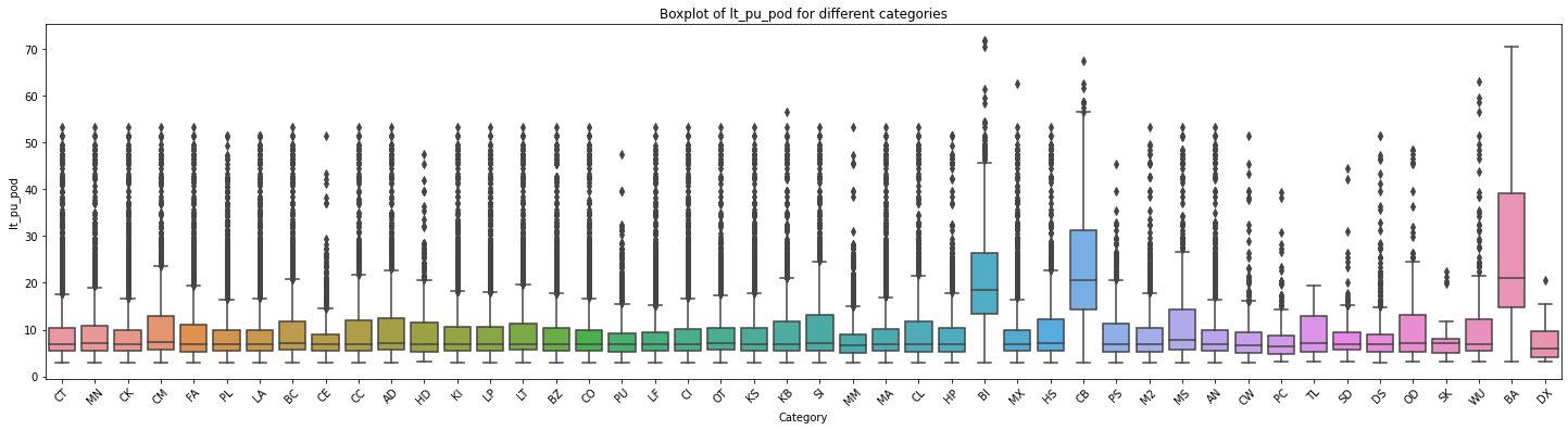
F统计量: 165.67483191021196
p值: 0.0
方差5、isgreen与LT_PU_POD的关联性
df_replen_1.groupby(['isgreen']).agg({'lt_pu_pod':['std','count','mean',lambda x:x.quantile(0.5),lambda x:x.quantile(0.9),lambda x:x.quantile(0.1)]}).reset_index()
| isgreen | lt_pu_pod | ||||||
|---|---|---|---|---|---|---|---|
| std | count | mean | <lambda_0> | <lambda_1> | <lambda_2> | ||
| 0 | GL1 | 6.818674 | 5810 | 10.340127 | 7.55 | 20.31 | 5.05 |
| 1 | GL2 | 0.836612 | 6 | 4.210000 | 4.74 | 4.76 | 3.13 |
# 创建一个空列表用于存储各个分类的数据
data_list = []

# 遍历每个分类,提取对应的数据并添加到列表中
for category in df_replen_1['isgreen'].unique().tolist():
    category_data = df_replen_1[df_replen_1['isgreen'] == category]['lt_pu_pod']
    data_list.append(category_data)

# 绘制箱线图
plt.figure(figsize=(25, 6))
sns.boxplot(data=data_list)
plt.xlabel('Category')
plt.ylabel('lt_pu_pod')
plt.title('Boxplot of lt_pu_pod for different categories')
plt.xticks(range(len(df_replen_1['isgreen'].unique().tolist())), df_replen_1['isgreen'].unique().tolist(),rotation=45)
plt.show()

# 执行方差分析
f_stat, p_value = f_oneway(*data_list)

# 输出结果
print("F统计量:", f_stat)
print("p值:", p_value)
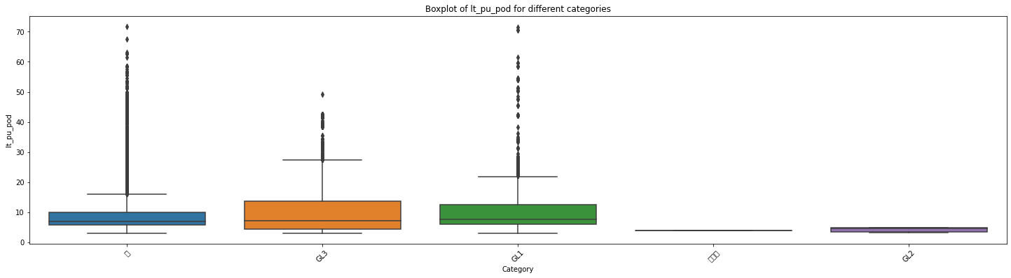
F统计量: 49.45782385934109
p值: 1.2062238051192215e-41
方差6、shippingfrequency与LT_PU_POD的关联性
df_replen_1.groupby(['shippingfrequency']).agg({'lt_pu_pod':['std','count','mean',lambda x:x.quantile(0.5),lambda x:x.quantile(0.9),lambda x:x.quantile(0.1)]}).reset_index()
| shippingfrequency | lt_pu_pod | ||||||
|---|---|---|---|---|---|---|---|
| std | count | mean | <lambda_0> | <lambda_1> | <lambda_2> | ||
| 0 | Bi-Weekly(Thu) | 17.664727 | 130 | 24.453231 | 15.940 | 54.18 | 9.731 |
| 1 | Bi-Weekly(Tue) | 9.306314 | 29 | 36.938276 | 35.590 | 49.57 | 23.954 |
| 2 | Bi-Weekly(Wed) | 2.271108 | 16 | 4.734375 | 3.840 | 5.48 | 3.820 |
| 3 | Daily | 6.448783 | 35322 | 7.890003 | 6.760 | 10.38 | 4.400 |
from scipy.stats import f_oneway

# 创建一个空列表用于存储各个分类的数据
data_list = []

# 遍历每个分类,提取对应的数据并添加到列表中
for category in df_replen_1['shippingfrequency'].unique().tolist():
    category_data = df_replen_1[df_replen_1['shippingfrequency'] == category]['lt_pu_pod']
    data_list.append(category_data)

# 绘制箱线图
plt.figure(figsize=(25, 6))
sns.boxplot(data=data_list)
plt.xlabel('Category')
plt.ylabel('lt_pu_pod')
plt.title('Boxplot of lt_pu_pod for different categories')
plt.xticks(range(len(df_replen_1['shippingfrequency'].unique().tolist())), df_replen_1['shippingfrequency'].unique().tolist(),rotation=45)
plt.show()

# 执行方差分析
f_stat, p_value = f_oneway(*data_list)

# 输出结果
print("F统计量:", f_stat)
print("p值:", p_value)
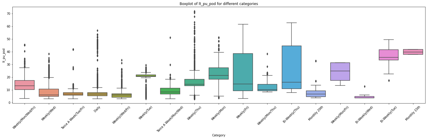
F统计量: 2693.5635083145007
p值: 0.0
方差7、forwarder与LT_PU_POD的关联性
# 创建一个空列表用于存储各个分类的数据
data_list = []

# 遍历每个分类,提取对应的数据并添加到列表中
for category in df_replen_1['forwarder'].unique().tolist():
    category_data = df_replen_1[df_replen_1['forwarder'] == category]['lt_pu_pod']
    data_list.append(category_data)

# 绘制箱线图
plt.figure(figsize=(25, 6))
sns.boxplot(data=data_list)
plt.xlabel('Category')
plt.ylabel('lt_pu_pod')
plt.title('Boxplot of lt_pu_pod for different categories')
plt.xticks(range(len(df_replen_1['forwarder'].unique().tolist())), df_replen_1['forwarder'].unique().tolist(),rotation=45)
plt.show()

# 执行方差分析
f_stat, p_value = f_oneway(*data_list)

# 输出结果
print("F统计量:", f_stat)
print("p值:", p_value)
F统计量: 12060.165772842343
p值: 0.0
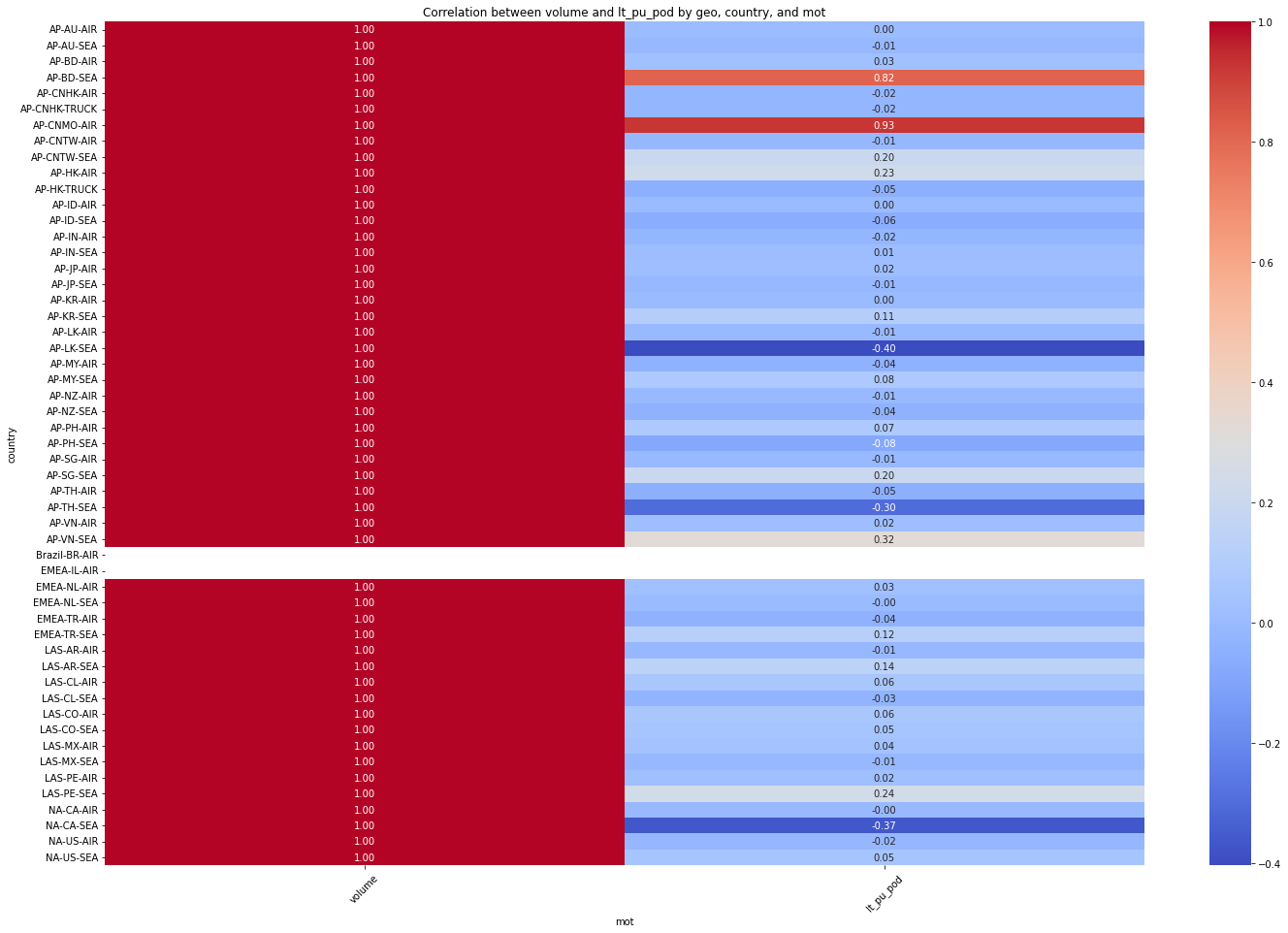
import pandas as pd
import seaborn as sns
import matplotlib.pyplot as plt

# 选择需要的特征列
cols = ['geo', 'country', 'mot', 'volume', 'lt_pu_pod']

# 提取对应的数据子集
data_subset = df_replen_1[cols]

# 计算每个geo下每个country和每个mot的volume与lt_pu_pod的相关性
correlation_matrix = data_subset.groupby(['geo', 'country', 'mot']).corr().loc[:, 'volume'].unstack()

# 绘制热力图
plt.figure(figsize=(24, 16))
sns.heatmap(data=correlation_matrix, cmap='coolwarm', annot=True, fmt=".2f", cbar=True)
plt.title("Correlation between volume and lt_pu_pod by geo, country, and mot")
plt.xlabel("mot")
plt.ylabel("country")
plt.xticks(rotation=45)
plt.show()
Step 5:Research climate<_pu_atd
df_replen_2 = df_replen_1.copy()
df_replen_2['ts_pu_date'] = df_replen_2['ts_pu'].map(lambda x:pd.to_datetime(x).strftime('%Y-%m-%d'))
df_replen_open['ts_pu_date'] = df_replen_open['ts_pu'].map(lambda x:pd.to_datetime(x).strftime('%Y-%m-%d'))
for rep_index in df_replen_2.index:
    ts_pu = (pd.to_datetime(df_replen_2.loc[rep_index,'ts_atd_pre_2_date']))
    ts_atd = (pd.to_datetime(df_replen_2.loc[rep_index,'ts_atd']))
    if pd.isna(ts_atd)==False:
        if ts_pu > ts_atd:
#             print(rep_index)
            ts_atd = (pd.to_datetime(df_replen_2.loc[rep_index,'ts_pu']) + datetime.timedelta(1.5))
    if pd.isna(ts_atd):
        ts_atd = (pd.to_datetime(df_replen_2.loc[rep_index,'ts_pu']) + datetime.timedelta(1.5))
    df_climate_tmp = df_climate_workday[(df_climate_workday['Date']<=ts_atd) & (df_climate_workday['Date']>=ts_pu)]
    holiday_count = len(df_climate_tmp[df_climate_tmp['weekday_cat']=='holiday'])
    climate_count = len(df_climate_tmp[df_climate_tmp['Alarm_info_cat']=='Abnormal climate'])
    # 判断期间有多少天假期
    if holiday_count == 0:
        df_replen_2.loc[rep_index,'holiday_count'] = '^== 0 hldys'
    if holiday_count == 1:
        df_replen_2.loc[rep_index,'holiday_count'] = '^== 1 hldys'
    if holiday_count == 2:
        df_replen_2.loc[rep_index,'holiday_count'] = '^== 2 hldys'
    if holiday_count > 2 and holiday_count <=7:
        df_replen_2.loc[rep_index,'holiday_count'] = '^<= 7 hldys'
    if holiday_count > 7 and holiday_count <=14:
        df_replen_2.loc[rep_index,'holiday_count'] = '^<= 14 hldys'
    if holiday_count > 14:
        df_replen_2.loc[rep_index,'holiday_count'] = '^> 14 hldys'

    # 判断期间有多少天恶劣天气
    if climate_count == 0:
        df_replen_2.loc[rep_index,'climate_count'] = '^== 0 abnr'
    if climate_count == 1:
        df_replen_2.loc[rep_index,'climate_count'] = '^== 1 abnr'
    if climate_count == 2:
        df_replen_2.loc[rep_index,'climate_count'] = '^== 2 abnr'
    if climate_count > 2 and climate_count <=7:
        df_replen_2.loc[rep_index,'climate_count'] = '^<= 7 abnr'
    if climate_count > 7 and climate_count <=14:
        df_replen_2.loc[rep_index,'climate_count'] = '^<= 14 abnr'
    if climate_count > 14:
        df_replen_2.loc[rep_index,'climate_count'] = '^> 14 abnr'
for rep_index in df_replen_open.index:
    ts_pu = (pd.to_datetime(df_replen_open.loc[rep_index,'ts_atd_pre_2_date']))
    ts_atd = (pd.to_datetime(df_replen_open.loc[rep_index,'ts_atd']))
    if pd.isna(ts_atd)==False:
        if ts_pu > ts_atd:
#             print(rep_index)
            ts_atd = (pd.to_datetime(df_replen_open.loc[rep_index,'ts_pu']) + datetime.timedelta(1.5))
    if pd.isna(ts_atd):
        ts_atd = (pd.to_datetime(df_replen_open.loc[rep_index,'ts_pu']) + datetime.timedelta(1.5))
    df_climate_tmp = df_climate_workday[(df_climate_workday['Date']<=ts_atd) & (df_climate_workday['Date']>=ts_pu)]
    holiday_count = len(df_climate_tmp[df_climate_tmp['weekday_cat']=='holiday'])
    climate_count = len(df_climate_tmp[df_climate_tmp['Alarm_info_cat']=='Abnormal climate'])
    # 判断期间有多少天假期
    if holiday_count == 0:
        df_replen_open.loc[rep_index,'holiday_count'] = '^== 0 hldys'
    if holiday_count == 1:
        df_replen_open.loc[rep_index,'holiday_count'] = '^== 1 hldys'
    if holiday_count == 2:
        df_replen_open.loc[rep_index,'holiday_count'] = '^== 2 hldys'
    if holiday_count > 2 and holiday_count <=7:
        df_replen_open.loc[rep_index,'holiday_count'] = '^<= 7 hldys'
    if holiday_count > 7 and holiday_count <=14:
        df_replen_open.loc[rep_index,'holiday_count'] = '^<= 14 hldys'
    if holiday_count > 14:
        df_replen_open.loc[rep_index,'holiday_count'] = '^> 14 hldys'

    # 判断期间有多少天恶劣天气
    if climate_count == 0:
        df_replen_open.loc[rep_index,'climate_count'] = '^== 0 abnr'
    if climate_count == 1:
        df_replen_open.loc[rep_index,'climate_count'] = '^== 1 abnr'
    if climate_count == 2:
        df_replen_open.loc[rep_index,'climate_count'] = '^== 2 abnr'
    if climate_count > 2 and climate_count <=7:
        df_replen_open.loc[rep_index,'climate_count'] = '^<= 7 abnr'
    if climate_count > 7 and climate_count <=14:
        df_replen_open.loc[rep_index,'climate_count'] = '^<= 14 abnr'
    if climate_count > 14:
        df_replen_open.loc[rep_index,'climate_count'] = '^> 14 abnr'
df_replen_2.groupby(['holiday_count']).agg({'lt_pu_atd':['std','count','mean',lambda x:x.quantile(0.5),lambda x:x.quantile(0.9),lambda x:x.quantile(0.1)]}).reset_index()
| holiday_count | lt_pu_atd | ||||||
|---|---|---|---|---|---|---|---|
| std | count | mean | <lambda_0> | <lambda_1> | <lambda_2> | ||
| 0 | ^<= 7 hldys | 2.053809 | 2204 | 4.793593 | 4.40 | 7.54 | 2.82 |
| 1 | ^== 0 hldys | 2.184254 | 52896 | 2.649606 | 2.12 | 5.44 | 0.44 |
| 2 | ^== 1 hldys | 2.411114 | 28255 | 2.461888 | 2.11 | 4.61 | 0.47 |
| 3 | ^== 2 hldys | 1.749583 | 19811 | 3.293560 | 2.90 | 5.13 | 1.75 |
# 创建一个空列表用于存储各个分类的数据
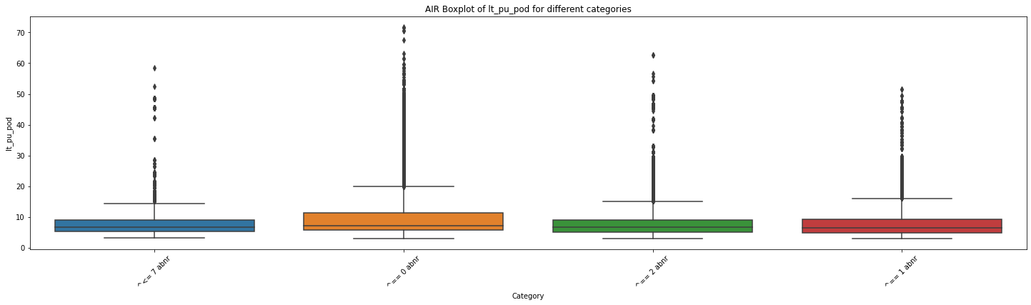
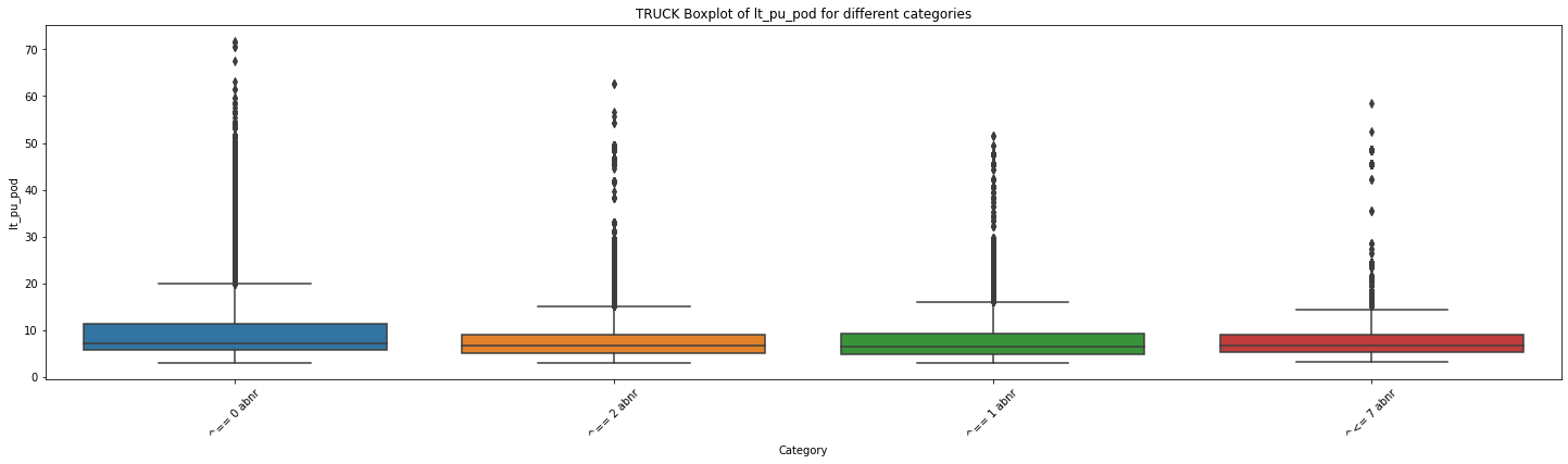
for mot in df_replen_2['mot'].unique().tolist():
# 遍历每个分类,提取对应的数据并添加到列表中
data_list = []
for category in df_replen_2[df_replen_2['mot']==mot]['climate_count'].unique().tolist():
category_data = df_replen_2[df_replen_2['climate_count'] == category]['lt_pu_pod']
data_list.append(category_data)
# 绘制箱线图
plt.figure(figsize=(25, 6))
sns.boxplot(data=data_list)
plt.xlabel('Category')
plt.ylabel('lt_pu_pod')
plt.title('{0} Boxplot of lt_pu_pod for different categories'.format(mot))
plt.xticks(range(len(df_replen_2[df_replen_2['mot']==mot]['climate_count'].unique().tolist())), df_replen_2[df_replen_2['mot']==mot]['climate_count'].unique().tolist(),rotation=45)
plt.show()
# 执行方差分析
f_stat, p_value = f_oneway(*data_list)
# 输出结果
print("F统计量:", f_stat)
print("p值:", p_value)
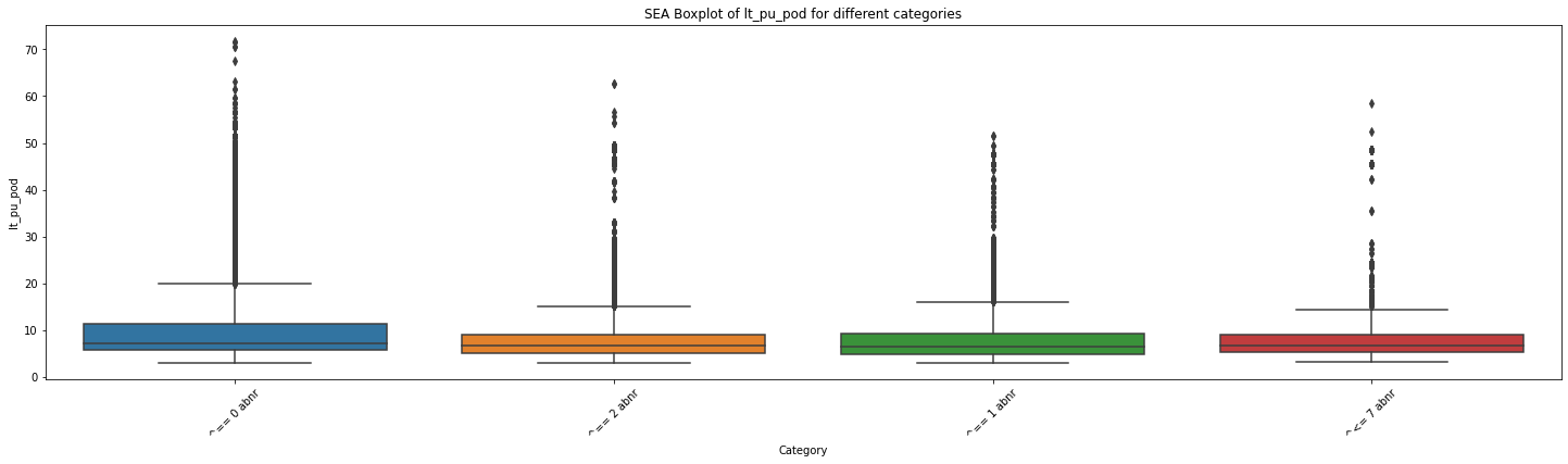
F统计量: 168.19664286910245
p值: 8.91244672555718e-109
F统计量: 168.19664286910245
p值: 8.91244672555718e-109
F统计量: 168.19664286910245
p值: 8.91244672555718e-109
import matplotlib.pyplot as plt
import seaborn as sns
# 创建一个空列表用于存储各个分类的数据
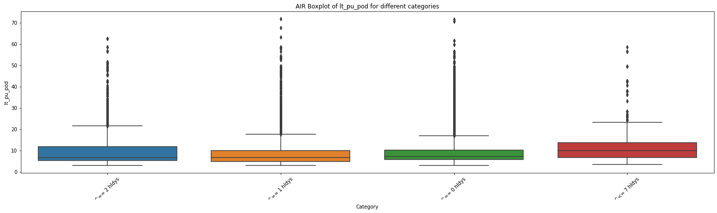
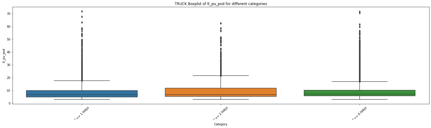
for mot in df_replen_2['mot'].unique().tolist():
# 遍历每个分类,提取对应的数据并添加到列表中
data_list = []
for category in df_replen_2[df_replen_2['mot']==mot]['holiday_count'].unique().tolist():
category_data = df_replen_2[df_replen_2['holiday_count'] == category]['lt_pu_pod']
data_list.append(category_data)
# 绘制箱线图
plt.figure(figsize=(25, 6))
sns.boxplot(data=data_list)
plt.xlabel('Category')
plt.ylabel('lt_pu_pod')
plt.title('{0} Boxplot of lt_pu_pod for different categories'.format(mot))
plt.xticks(range(len(df_replen_2[df_replen_2['mot']==mot]['holiday_count'].unique().tolist())), df_replen_2[df_replen_2['mot']==mot]['holiday_count'].unique().tolist(),rotation=45)
plt.show()
# 执行方差分析
f_stat, p_value = f_oneway(*data_list)
# 输出结果
print("F统计量:", f_stat)
print("p值:", p_value)
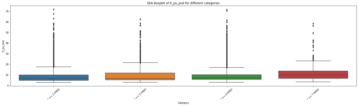
F统计量: 134.89417962378948
p值: 3.1763774706854116e-87
F统计量: 134.89417962378948
p值: 3.1763774706854116e-87
F统计量: 82.45295180623998
p值: 1.6609295478352026e-36
df_replen_2['ts_pu_date'] = pd.to_datetime(df_replen_2['ts_pu_date'])
df_replen_open['ts_pu_date'] = pd.to_datetime(df_replen_open['ts_pu_date'])
df_replen_2 = pd.merge(df_replen_2,df_climate_workday[['Date','Alarm_info_cat','weekday_cat','Week','weekday']],left_on='ts_pu_date',right_on='Date',how='left').drop('Date',axis=1).rename(columns={'天气':'climate','分类':'climate_category'})
df_replen_open = pd.merge(df_replen_open,df_climate_workday[['Date','Alarm_info_cat','weekday_cat','Week','weekday']],left_on='ts_pu_date',right_on='Date',how='left').drop('Date',axis=1).rename(columns={'天气':'climate','分类':'climate_category'})
df_replen_2['lt_pu_ata'] = (pd.to_datetime(df_replen_1['ts_ata']) - pd.to_datetime(df_replen_1['ts_pu'])).astype('timedelta64[D]').astype(float)
df_replen_2['lt_pu_atd'] = (pd.to_datetime(df_replen_1['ts_atd']) - pd.to_datetime(df_replen_1['ts_pu'])).astype('timedelta64[D]').astype(float)
df_climate_workday
| Date | Week | maximum_temperature | minimum_temperature | climate | wind_direction | city | is_workday | is_holiday | holiday_name | weekday | weekday_cat | date_alarm | Alarm_info | Alarm_info_cat | unic_version | rank_1 | |
|---|---|---|---|---|---|---|---|---|---|---|---|---|---|---|---|---|---|
| 0 | 2022-01-01 | 星期六 | 0℃ | -9℃ | 多云 | 西风 2级 | 上海 | 0 | 1 | New year | 5 | holiday | NaT | None | None | 2023-05-18 16:25:25 | 1 |
| 1 | 2022-01-02 | 星期日 | 8℃ | -4℃ | 多云 | 西风 3级 | 上海 | 0 | 0 | 6 | holiday | NaT | None | None | 2023-05-18 16:25:25 | 1 | |
| 2 | 2022-01-03 | 星期一 | 13℃ | 6℃ | 晴 | 东南风 2级 | 上海 | 0 | 1 | New Year shift | 0 | holiday | NaT | None | None | 2023-05-18 16:25:25 | 1 |
| 3 | 2022-01-04 | 星期二 | 13℃ | 9℃ | 多云 | 东北风 1级 | 上海 | 1 | 0 | 1 | workday | NaT | None | None | 2023-05-18 16:25:25 | 1 |
502 rows × 17 columns
# 创建一个空列表用于存储各个分类的数据
for mot in df_replen_2['mot'].unique().tolist():
    # 遍历每个分类,提取对应的数据并添加到列表中
    data_list = []
    for category in df_replen_2[(df_replen_2['mot']==mot) & (~df_replen_2['weekday'].isnull())]['weekday'].unique().tolist():
        category_data = df_replen_2[(df_replen_2['mot']==mot) & (~df_replen_2['weekday'].isnull()) & (df_replen_2['weekday'] == category)]['lt_pu_pod']
        data_list.append(category_data)

    # 绘制箱线图
    plt.figure(figsize=(25, 6))
    sns.boxplot(data=data_list)
    plt.xlabel('Category')
    plt.ylabel('lt_pu_pod')
    plt.title('{0} Boxplot of lt_pu_pod for different categories'.format(mot))
    plt.xticks(range(len(df_replen_2[df_replen_2['mot']==mot]['weekday'].unique().tolist())), df_replen_2[df_replen_2['mot']==mot]['weekday'].unique().tolist(),rotation=45)
    plt.show()

    # 执行方差分析
    f_stat, p_value = f_oneway(*data_list)

    # 输出结果
    print("F统计量:", f_stat)
    print("p值:", p_value)
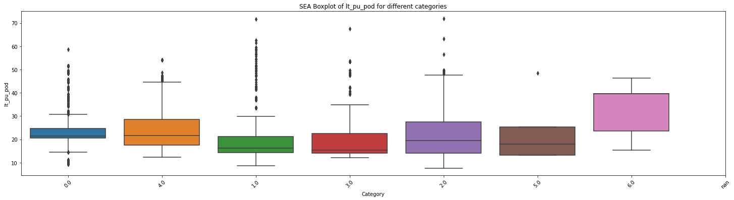
F统计量: 127.26212162797701
p值: 4.906400437665232e-156
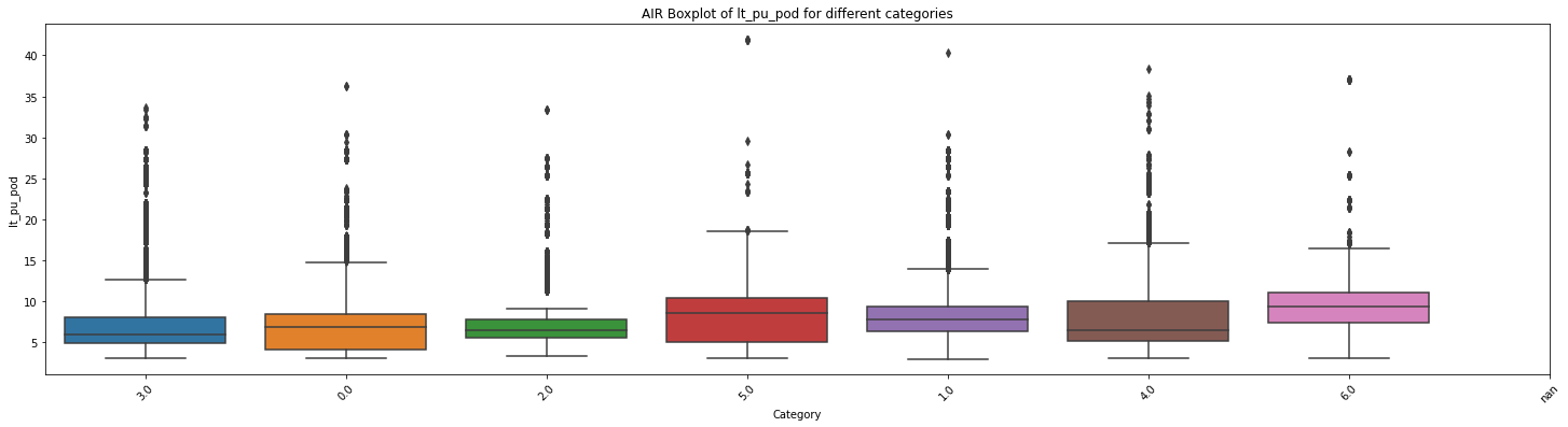
F统计量: 326.9319114756572
p值: 0.0
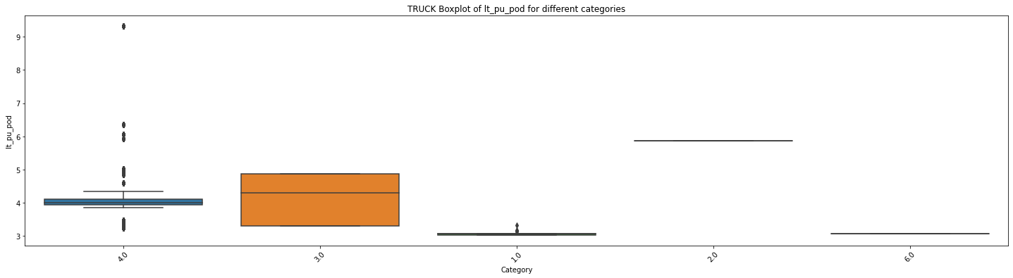
F统计量: 52.61132203829418
p值: 1.6153144700352586e-42
group_mot_climate_pu_atd = df_replen_2.groupby(['mot','Week']).agg({'lt_pu_atd':['std','count','mean',lambda x:x.quantile(0.5),lambda x:x.quantile(0.9),lambda x:x.quantile(0.1)]}).reset_index()
group_mot_climate_pu_atd.columns = ['mot','holiday_count','std','count','mean','quantile_5','quantile_9','quantile_1']
group_mot_climate_pu_atd
| mot | holiday_count | std | count | mean | quantile_5 | quantile_9 | quantile_1 | |
|---|---|---|---|---|---|---|---|---|
| 0 | AIR | 星期一 | 1.547858 | 16544 | 1.896216 | 2.0 | 4.0 | 0.0 |
| 1 | AIR | 星期三 | 1.566505 | 15121 | 2.017195 | 2.0 | 4.0 | 0.0 |
| 2 | AIR | 星期二 | 1.751875 | 17681 | 2.023698 | 2.0 | 4.0 | 0.0 |
| 3 | AIR | 星期五 | 2.986730 | 12385 | 2.426968 | 2.0 | 6.0 | 0.0 |
group_mot_climate_pu_atd = df_replen_2.groupby(['mot','holiday_count']).agg({'lt_pu_atd':['std','count','mean',lambda x:x.quantile(0.5),lambda x:x.quantile(0.9),lambda x:x.quantile(0.1)]}).reset_index()
group_mot_climate_pu_atd.columns = ['mot','holiday_count','std','count','mean','quantile_5','quantile_9','quantile_1']
group_mot_climate_pu_atd
| mot | holiday_count | std | count | mean | quantile_5 | quantile_9 | quantile_1 | |
|---|---|---|---|---|---|---|---|---|
| 0 | AIR | ^<= 7 hldys | 1.945878 | 1761 | 4.040318 | 4.0 | 7.0 | 2.0 |
| 1 | AIR | ^== 0 hldys | 1.994225 | 46645 | 2.012199 | 1.0 | 5.0 | 0.0 |
| 2 | AIR | ^== 1 hldys | 2.298573 | 24303 | 1.870139 | 2.0 | 4.0 | 0.0 |
| 3 | AIR | ^== 2 hldys | 1.453881 | 17330 | 2.536411 | 2.0 | 4.0 | 1.0 |
| 4 | SEA | ^<= 7 hldys | 2.124920 | 443 | 5.316027 | 6.0 | 7.0 | 2.0 |
group_mot_climate_pu_atd = df_replen_2.groupby(['mot','climate_count']).agg({'lt_pu_atd':['std','count','mean',lambda x:x.quantile(0.5),lambda x:x.quantile(0.9),lambda x:x.quantile(0.1)]}).reset_index()
group_mot_climate_pu_atd.columns = ['mot','climate_count','std','count','mean','quantile_5','quantile_9','quantile_1']
group_mot_climate_pu_atd
| mot | climate_count | std | count | mean | quantile_5 | quantile_9 | quantile_1 | |
|---|---|---|---|---|---|---|---|---|
| 0 | AIR | ^<= 7 abnr | 1.187565 | 3495 | 1.614878 | 1.0 | 3.0 | 0.0 |
| 1 | AIR | ^== 0 abnr | 2.271866 | 62167 | 2.280551 | 2.0 | 5.0 | 0.0 |
| 2 | AIR | ^== 1 abnr | 1.276714 | 12195 | 1.778598 | 2.0 | 3.0 | 0.0 |
| 3 | AIR | ^== 2 abnr | 1.197433 | 12182 | 1.746101 | 2.0 | 3.0 | 0.0 |
group_mot_climate_pu_atd = df_replen_2.groupby(['mot','climate_count','holiday_count']).agg({'lt_pu_atd':['std','count','mean',lambda x:x.quantile(0.5),lambda x:x.quantile(0.9),lambda x:x.quantile(0.1)]}).reset_index()
group_mot_climate_pu_atd.columns = ['mot','climate_count','holiday_count','std','count','mean','quantile_5','quantile_9','quantile_1']
group_mot_climate_pu_atd.sort_values('mean',ascending=False)
| mot | climate_count | holiday_count | std | count | mean | quantile_5 | quantile_9 | quantile_1 | |
|---|---|---|---|---|---|---|---|---|---|
| 17 | SEA | ^== 0 abnr | ^<= 7 hldys | 1.830452 | 272 | 6.000000 | 7.0 | 7.0 | 2.2 |
df_replen_2['ts_pu'] = pd.to_datetime((df_replen_2['ts_pu']))
df_replen_open['ts_pu'] = pd.to_datetime((df_replen_open['ts_pu']))
df_replen_2['ts_pu_hour'] = df_replen_2['ts_pu'].dt.hour
df_replen_open['ts_pu_hour'] = df_replen_open['ts_pu'].dt.hour
df_replen_2['dayofweek'] = df_replen_2['ts_pu'].dt.dayofweek
df_replen_open['dayofweek'] = df_replen_open['ts_pu'].dt.dayofweek
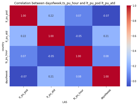
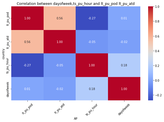
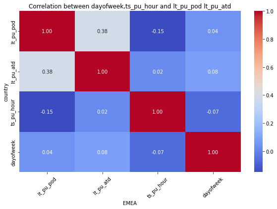
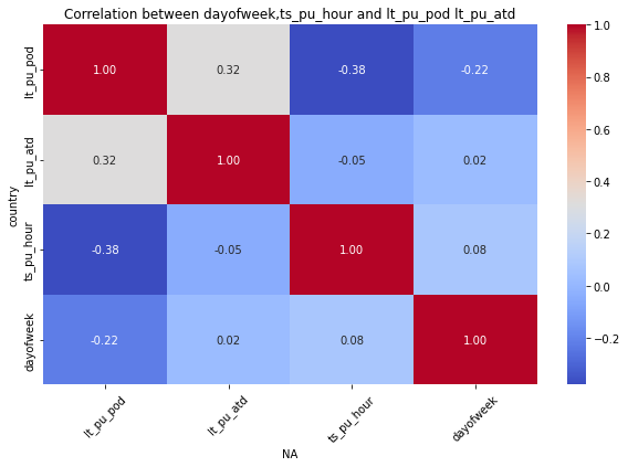
for mot in df_replen_2['geo'].unique().tolist():
    plt.figure(figsize=(10, 6))
    sns.heatmap(data=df_replen_2[(df_replen_2['geo']==mot)][['lt_pu_pod','lt_pu_atd','ts_pu_hour','dayofweek']].corr(), cmap='coolwarm', annot=True, fmt=".2f", cbar=True)
    plt.title("Correlation between dayofweek,ts_pu_hour and lt_pu_pod lt_pu_atd")
    plt.xlabel("{0}".format(mot))
    plt.ylabel("country")
    plt.xticks(rotation=45)
    plt.show()