1 Introduction
1.1 定义
定义:
Dynamic: sequential or temporal component to the problem
Programming: optimising a program: a policy
核心思想:
将复杂问题拆解成简单子问题
1.2 Requirements for dynamic programming
- Optimal substructure
- principle of optimality applies
- optimal solution can be decomposed into subproblems
- overlapping subproblems
- subproblem会调用很多次
- solution需要存储起来和进行复用
- MDP 满足以下性质
- bellman 方程提供递归的分解
- value 函数存储和复用solutions
1.3 planning by dynamic programming
几种假设:
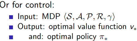
1)DP 假设对MDP可观测结果
2)for prediction

3)for control
1.4 动态规划的其他应用
- Scheduling algorithm
- String algorithms (e.g. sequence alignment)
- Graph algorithms (e.g. shortest path algorithms)
- Graphical models (e.g. Viterbi algorithm)
- Bioinformatics (e.g. lattice models)
2 Policy Evaluation
动态问题的结构可以拆成下面三个部分:
state transition
s
n
=
f
(
s
n
−
1
,
a
n
)
value function
J
∗
(
s
)
=
min
a
∈
A
{
l
(
s
,
a
)
+
γ
∑
s
′
∈
S
P
(
s
′
∣
s
,
a
)
J
∗
(
s
′
)
}
policy
π
(
s
)
=
arg
min
a
{
l
(
s
,
a
)
+
γ
∑
s
′
∈
S
P
(
s
′
∣
s
,
a
)
J
∗
(
s
′
)
}
\begin{aligned} \text{state transition} & \quad s_{n} = f(s_{n-1}, a_{n}) \\ \text{value function} & \quad J^*(s) = \min \limits_{a\in A} \{l(s,a)+\gamma \sum_{s' \in S} P(s' | s, a) J^*(s')\} \\ \text{policy} & \quad \pi(s)=\arg\min \limits_{a} \{l(s,a)+\gamma \sum_{s' \in S} P(s' | s, a) J^*(s')\} \end{aligned}
state transitionvalue functionpolicysn=f(sn−1,an)J∗(s)=a∈Amin{l(s,a)+γs′∈S∑P(s′∣s,a)J∗(s′)}π(s)=argamin{l(s,a)+γs′∈S∑P(s′∣s,a)J∗(s′)}
代码的结构大概是这样的
```matlab
for state = 1:num_state
	for action = 1:nun_action
		Q = instaneous_cost(state, action);
		next_state = transition(state, action);
		Q = Q + J(next_state);
	end
end
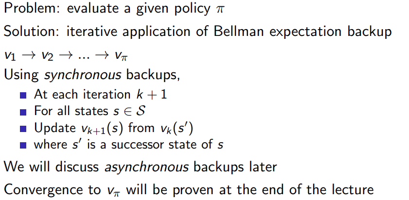
用iterative policy Evaluation 表示:
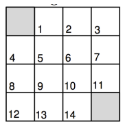
解决一个gridworld的问题,首先,我们定义一个简化的 4x4 网格世界,其中有四个可能的动作:向上、向下、向左、向右。在这个示例中,我们将使用均匀随机策略,即在每个状态下,每个动作的概率都相等。
% Initialize the grid world and parameters
grid_size = 4;
num_actions = 4;
discount_factor = 1.0;
theta = 1e-4;

% Initialize state-value function
V = zeros(grid_size);

% Define the reward function
reward = -1;

% Define the transition probabilities for the uniform random policy
policy = ones(grid_size, grid_size, num_actions) / num_actions;

% Iterative Policy Evaluation
while true
    delta = 0;

    % Loop over all states
    for i = 1:grid_size
        for j = 1:grid_size

            % Skip the start and terminal states
            if (i == 1 && j == 1) || (i == grid_size && j == grid_size)
                continue;
            end

            % Store the old value
            old_value = V(i, j);

            % Calculate the new value by averaging over actions
            new_value = 0;
            for action = 1:num_actions
                [next_i, next_j] = apply_action(i, j, action);
                reward_next = (next_i == grid_size && next_j == grid_size) * (1 - discount_factor);
                new_value = new_value + policy(i, j, action) * (reward + reward_next + discount_factor * V(next_i, next_j));
            end

            % Update the value function
            V(i, j) = new_value;
            delta = max(delta, abs(old_value - new_value));
        end
    end

    % Check for convergence
    if delta < theta
        break;
    end
end

% Apply the given action to the current state (i, j)
function [next_i, next_j] = apply_action(i, j, action)
    grid_size = 4;

    % Actions: 1 = up, 2 = down, 3 = left, 4 = right
    if action == 1
        next_i = max(i - 1, 1);
        next_j = j;
    elseif action == 2
        next_i = min(i + 1, grid_size);
        next_j = j;
    elseif action == 3
        next_i = i;
        next_j = max(j - 1, 1);
    else
        next_i = i;
        next_j = min(j + 1, grid_size);
    end
end
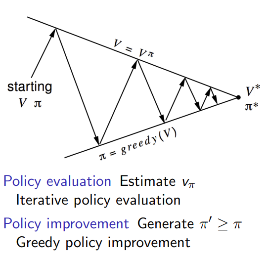
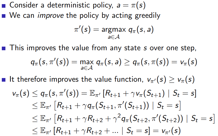
3 policy Iteration
3.1 how to improve policy
Give a policy π \pi π
- Evaluate the policy π \pi π
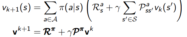
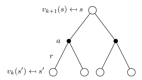
V π ( s ) = ∑ a ∈ A π ( a ∣ s ) [ R ( s , a ) + γ ∑ s ′ ∈ S P ( s ′ ∣ s , a ) V π ( s ′ ) ] V_{\pi}(s) = \sum_{a \in \mathcal{A}} \pi(a|s) \left[R(s, a) + \gamma \sum_{s' \in \mathcal{S}} P(s'|s, a) V_{\pi}(s')\right] Vπ(s)=a∈A∑π(a∣s)[R(s,a)+γs′∈S∑P(s′∣s,a)Vπ(s′)]
Improve the policy by acting greedily with respect to v π v_{\pi} vπ
π ′ = g r e e d y ( v π ) \pi'=greedy(v_{\pi}) π′=greedy(vπ)
每一步都找出optimal的value function, 作为state的value function
这里我们将使用一个简单的网格世界(Grid World)环境作为Policy Iteration的范例。这个环境中,智能体(agent)可以执行四个操作:上、下、左、右。智能体的目标是从初始位置移动到终点位置,同时最小化行动次数。
假设我们有一个4x4的网格世界,终点位置在右下角。每次行动的奖励(reward)是-1。使用Policy Iteration方法,我们将找到一个策略,使得智能体以最少的行动次数到达终点。
import numpy as np

def gridworld_policy_iteration():
    n_states = 16
    n_actions = 4
    terminal_state = 15
    rewards = -1 * np.ones((n_states, n_actions))
    rewards[terminal_state, :] = 0

    transition_matrix = np.zeros((n_states, n_actions, n_states))

    for state in range(n_states):
        for action in range(n_actions):
            if state == terminal_state:
                transition_matrix[state, action, state] = 1
                continue

            next_state = state

            if action == 0:  # Up
                next_state = max(state - 4, 0)
            elif action == 1:  # Down
                next_state = min(state + 4, n_states - 1)
            elif action == 2:  # Left
                next_state = state - 1
                if state % 4 == 0:
                    next_state = state
            elif action == 3:  # Right
                next_state = state + 1
                if (state + 1) % 4 == 0:
                    next_state = state

            transition_matrix[state, action, next_state] = 1

    gamma = 0.99
    max_iter = 1000
    theta = 1e-10

    policy = np.ones((n_states, n_actions)) / n_actions

    for _ in range(max_iter):
        policy_stable = True

        # Policy Evaluation
        V = np.zeros(n_states)
        while True:
            delta = 0
            for state in range(n_states):
                v = V[state]
                V[state] = np.sum(policy[state, :] * (rewards[state, :] + gamma * transition_matrix[state, :, :] @ V))
                delta = max(delta, abs(v - V[state]))
            if delta < theta:
                break

        # Policy Improvement
        for state in range(n_states):
            old_action = np.argmax(policy[state, :])
            action_returns = np.zeros(n_actions)
            for action in range(n_actions):
                action_returns[action] = rewards[state, action] + gamma * np.dot(transition_matrix[state, action, :], V)
            best_action = np.argmax(action_returns)
            policy[state, :] = 0
            policy[state, best_action] = 1

            if old_action != best_action:
                policy_stable = False

        if policy_stable:
            break

    optimal_policy = policy
    state_values = V

    return optimal_policy, state_values

optimal_policy, state_values = gridworld_policy_iteration()
print("Optimal Policy:")
print(optimal_policy)
print("State Values:")
print(state_values)
代码的关键在于
# 找到最大reward对应的action,对其policy为1,其他为0
            for action in range(n_actions):
                action_returns[action] = rewards[state, action] + gamma * np.dot(transition_matrix[state, action, :], V)
            best_action = np.argmax(action_returns)
            policy[state, :] = 0
            policy[state, best_action] = 1
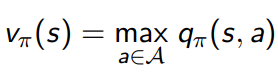
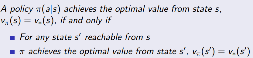
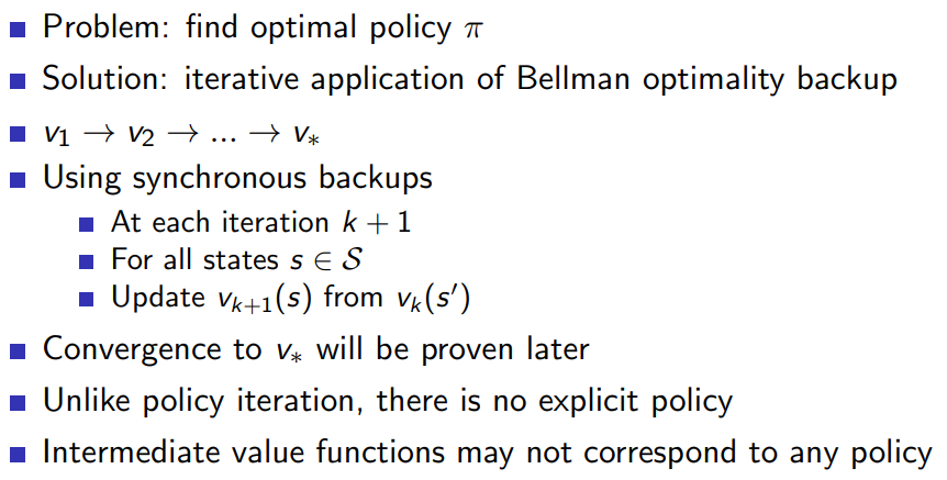
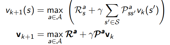
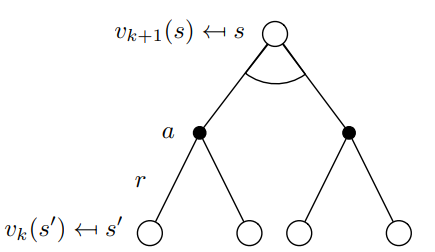
4 value iteration
4.1 value iteration in MDPs
4.1.1 principle of optimality
任何的优化策略可以划分成两个组成部分,
1.第一步采用最优动作
A
∗
A_{*}
A∗
2.对successor state采用optimal policy
4.1.2 deterministic value iteration
- 子问题的solution v ∗ ( s ′ ) v_{*}(s') v∗(s′)
- 问题的solution
v
∗
(
s
)
v_{*}(s)
v∗(s)可以通过往前走一步得到
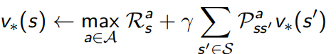
- 直觉理解,start with final rewards and work backwards
- still works with loopy, stochastic MDPs
值迭代的思想非常简单,代码看起来更美观一点
import numpy as np

# GridWorld environment
rows = 4
cols = 4
terminal_states = [(0, 0), (rows-1, cols-1)]
actions = [(0, 1), (1, 0), (0, -1), (-1, 0)]

def is_valid_state(state):
    r, c = state
    return 0 <= r < rows and 0 <= c < cols and state not in terminal_states

def next_state(state, action):
    r, c = np.array(state) + np.array(action)
    if is_valid_state((r, c)):
        return r, c
    return state

# Value iteration
def value_iteration(gamma=1, theta=1e-6):
    V = np.zeros((rows, cols))
    while True:
        delta = 0
        for r in range(rows):
            for c in range(cols):
                state = (r, c)
                if state in terminal_states:
                    continue

                v = V[state]
                max_value = float('-inf')
                for a in actions:
                    next_s = next_state(state, a)
                    value = -1 + gamma * V[next_s]
                    max_value = max(max_value, value)
                V[state] = max_value
                delta = max(delta, abs(v - V[state]))

        if delta < theta:
            break
    return V

# Find optimal policy
def find_optimal_policy(V, gamma=1):
    policy = np.zeros((rows, cols, len(actions)))
    for r in range(rows):
        for c in range(cols):
            state = (r, c)
            if state in terminal_states:
                continue

            q_values = np.zeros(len(actions))
            for i, a in enumerate(actions):
                next_s = next_state(state, a)
                q_values[i] = -1 + gamma * V[next_s]
            optimal_action = np.argmax(q_values)
            policy[state][optimal_action] = 1
    return policy

# Find the shortest path using the optimal policy
def find_shortest_path(policy):
    state = (0, 0)
    path = [state]
    while state != (rows-1, cols-1):
        action_idx = np.argmax(policy[state])
        state = next_state(state, actions[action_idx])
        path.append(state)
    return path

V = value_iteration()
policy = find_optimal_policy(V)
path = find_shortest_path(policy)

print("Shortest path:", path)
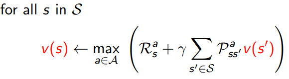
5 extensions to DP
5.1 Asynchronous Dynamic Programming
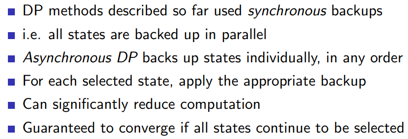

5.1.1 in place dynamic programming
- synchronuous value iteration
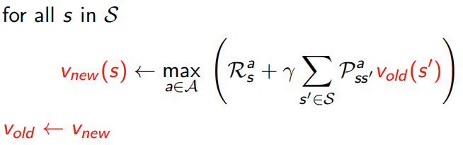
- in place value iteration
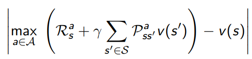
5.1.2 prioritised sweeping
- Use magnitude of Bellman error to guide state selection, e.g.
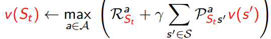
5.1.3 real time dp
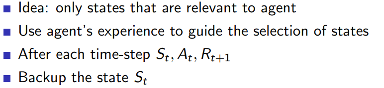
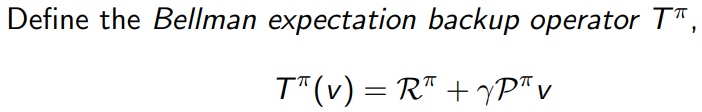
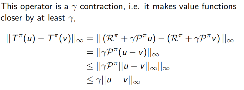
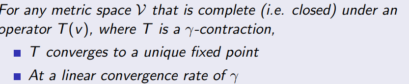
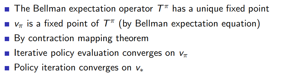
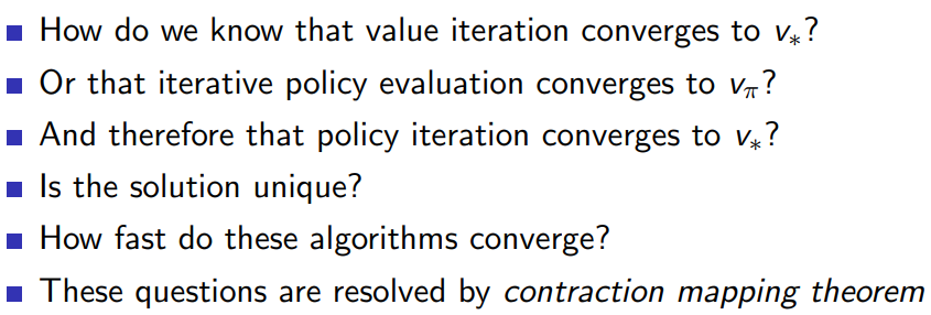
6 Contraction Mapping
类似于李雅普诺夫稳定性的定义
6.1技术问题
6.2 value function space
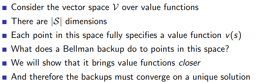
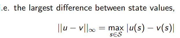
6.3 bellman expectation backup is a contraction