基于在线优化的快速模型预测控制仿真Fast

基于在线优化的快速模型预测控制仿真Fast_MPC（Matlab代码实现）

news2025/10/31 23:14:10

💥1 概述

📚2 运行结果

🎉3 参考文献

👨‍💻4 Matlab代码

💥1 概述

模型预测控制(Model Predictive Control,MPC)是一种基于在线计算的控制优化算法,能够统一处理带约束的多参数优化控制问题。当被控对象结构和环境相对复杂时,模型预测控制需选择较大的预测时域和控制时域,因此大大增加了在线求解的计算时间,同时降低了控制效果。从现有的算法来看,模型预测控制通常只适用于采样时间较大、动态过程变化较慢的系统中。因此,研究快速模型预测控制算法具有一定的理论意义和应用价值。

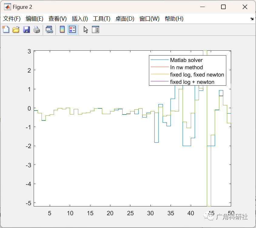
📚2 运行结果

主函数部分代码：

% Testing FAST MPC class
clear;
clc;
close all;
addpath('Fast_MPC');
%% Parameters

n = 8;                      % Dimension of state
m = 5;                      % Dimension of control
Q = eye(n);                 % State stage cost
R = eye(m);                 % Control stage cost
S = [];                     % State control coupled cost
Qf = 50*eye(n);             % Terminal state cost
q = [];                     % Linear state cost
r = [];                     % Linear control cost
qf = [];                    % Terminal state cost
Xmax = 10;                  % State upper limit
Umax = 2;                   % Control upper limit
xmin = -Xmax*ones(n,1);     % State lower bound
xmax = Xmax*ones(n,1);      % State upper bound
umin = -Umax*ones(m,1);     % Cotrol lower bound
umax = Umax*ones(m,1);      % Control upper bound

high_limit = 1;
low_limit = 0;
A = (high_limit-low_limit).*rand(n,n) + ones(n,n)*low_limit;    % Random A (State transition) matrix
B = (high_limit-low_limit).*rand(n,m) + ones(n,m)*low_limit;    % Random B (Control matrix) matrix

A = A./(max(abs(eig(A))));      % Spectral radius of A within 1

high_limit_w = 1;               
low_limit_w = 0;
w = (high_limit_w-low_limit_w).*rand(n,1) + ones(n,1)*low_limit_w;  % Random noise vector

T = 10;                         % Horizon length
x0 = rand(n,1);                 % Initial state (random)
xf = 1*ones(n,1);               % Terminal state
test = Fast_MPC2(Q,R,S,Qf,q,r,qf,xmin,xmax,umin,umax,T,x0,...
                A,B,w,xf,[]);   % Build class

%% Solve

% Native matlab solver
tic;
[x_opt_mat] = test.matlab_solve;            % Solving using native matlab solver fmincon
t_mat = toc;

% Structured MPC full solve
tic;
[x_opt_full] = test.mpc_solve_full;         % Solving structure problem as log barrier method with infeasible start newton
t_full = toc;

% Fixed log barrier method k=0.01
k_fix = 0.01;
tic;
[x_opt_log] = test.mpc_fixed_log(k_fix);     % Fixed log(k) iteration method
t_log = toc;

% Fixed newton step = 5
n_fix = 5;
tic;
[x_opt_nw] = test.mpc_fixed_newton(n_fix);       % Fixed newton steps(5) method
t_nw = toc;

% Fixed log barrier + fixed newton step
tic;
[x_opt_lgnw] = test.mpc_fixed_log_newton(n_fix,k_fix);
t_lgnw = toc;

fprintf('Matlab solver=%d sec\n',t_mat);
fprintf('Infeasible start newton =%d sec\n',t_full);
fprintf('Infeasible start newton with fixed k(%d) =%d sec\n',k_fix,t_log);
fprintf('Infeasible start newton with fixed newton step(%d) =%d sec\n',n_fix,t_nw);
fprintf('Infeasible start newton with fixed newton and barrier =%d sec\n',t_lgnw);

%% Plotting

x_mat = zeros(T*n,1);
u_mat = zeros(T*m,1);
for i=1:(m+n):length(x_opt_mat)
    if i==1
        u_mat(i:i+m-1) = x_opt_mat(i:i+m-1);
        x_mat(i:i+n-1) = x_opt_mat(i+m:i+m+n-1);
    else
        u_mat((i-1)/(m+n)*m+1:(i-1)/(m+n)*m+m) = x_opt_mat(i:i+m-1);
        x_mat((i-1)/(m+n)*n+1:(i-1)/(m+n)*n+n) = x_opt_mat(i+m:i+m+n-1);
    end
end

x_full = zeros(T*n,1);
u_full = zeros(T*m,1);
for i=1:(m+n):length(x_opt_full)
    if i==1
        u_full(i:i+m-1) = x_opt_full(i:i+m-1);
        x_full(i:i+n-1) = x_opt_full(i+m:i+m+n-1);
    else
        u_full((i-1)/(m+n)*m+1:(i-1)/(m+n)*m+m) = x_opt_full(i:i+m-1);
        x_full((i-1)/(m+n)*n+1:(i-1)/(m+n)*n+n) = x_opt_full(i+m:i+m+n-1);
    end
end

x_log = zeros(T*n,1);
u_log = zeros(T*m,1);
for i=1:(m+n):length(x_opt_log)
    if i==1
        u_log(i:i+m-1) = x_opt_log(i:i+m-1);
        x_log(i:i+n-1) = x_opt_log(i+m:i+m+n-1);
    else
        u_log((i-1)/(m+n)*m+1:(i-1)/(m+n)*m+m) = x_opt_log(i:i+m-1);
        x_log((i-1)/(m+n)*n+1:(i-1)/(m+n)*n+n) = x_opt_log(i+m:i+m+n-1);
    end
end