face3d: Python tools for processing 3D face
git code: https://github.com/yfeng95/face3d
paper list: PaperWithCode
基于BFM模型,估计3DMM的参数,可以实现线性的人脸表征,该方法可用于基于关键点的人脸生成、位姿检测以及渲染等。推荐!!!
目录
- face3d: Python tools for processing 3D face
- 一、回顾
- 1.1 将(2)中求出的 s , R , t 2 d s,R,t_{2d} s,R,t2d 带入能量方程,解得β
- 1.2 (4).将(2)和(3)中求出的β代入能量方程,解得α
- 1.3 (5)更新α , β 的值,重复(2)-(4)进行迭代更新
- 总结
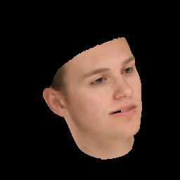
3DMM模型生成的人脸1:平常表情

3DMM模型生成的人脸2:微笑表情
3DMM模型是如何运行的?其原理是怎样的?如何实现三维人脸定制生成呢?
要回答上述问题,必须要弄清楚3DMM提供了哪些信息?如何编辑这些信息以达到特定的人脸生成。
一、回顾
在Face3d中的求解过程可以概述如下:
- 初始化α , β 为0;
- 利用黄金标准算法得到一个仿射矩阵{P_A},分解得到 s , R , t 2 d {s,R,t_{2d}} s,R,t2d
- 将(2)中求出的 s , R , t 2 d s,R,t_{2d} s,R,t2d 带入能量方程,解得β;
- 将(2)和(3)中求出的α代入能量方程,解得α;
- 更新α , β的值,重复(2)-(4)进行迭代更新
我们在上一个系列中已经介绍了算法的前两步骤。这里继续分析如何求解α , β
1.1 将(2)中求出的 s , R , t 2 d s,R,t_{2d} s,R,t2d 带入能量方程,解得β
代码分析
在上一篇文章我们通过黄金标准算法求解出了仿射矩阵
P
A
P_A
PA并将它分解的到了
s
,
R
,
t
2
d
s,R,t_{2d}
s,R,t2d,这部分将继续按照求解步骤进行源码分析:
for i in range(max_iter):
        X = shapeMU + shapePC.dot(sp) + expPC.dot(ep)
        X = np.reshape(X, [int(len(X)/3), 3]).T

        #----- estimate pose
        P = mesh.transform.estimate_affine_matrix_3d22d(X.T, x.T)
        s, R, t = mesh.transform.P2sRt(P)
        rx, ry, rz = mesh.transform.matrix2angle(R)
        # print('Iter:{}; estimated pose: s {}, rx {}, ry {}, rz {}, t1 {}, t2 {}'.format(i, s, rx, ry, rz, t[0], t[1]))

        #----- estimate shape
        # expression
        shape = shapePC.dot(sp)
        shape = np.reshape(shape, [int(len(shape)/3), 3]).T
        ep = estimate_expression(x, shapeMU, expPC, model['expEV'][:n_ep,:], shape, s, R, t[:2], lamb = 0.002)

        # shape
        expression = expPC.dot(ep)
        expression = np.reshape(expression, [int(len(expression)/3), 3]).T
        sp = estimate_shape(x, shapeMU, shapePC, model['shapeEV'][:n_sp,:], expression, s, R, t[:2], lamb = 0.004)

    return sp, ep, s, R, t
对于公式:

其中形状部分为
∑
i
=
1
m
α
i
S
i
\sum_{i=1}^{m}\alpha_iS_i
∑i=1mαiSi,通过
shape = shapePC.dot(sp)
来定义shape的加成。
shape的格式为(159645,1),再通过
shape = np.reshape(shape, [int(len(shape)/3), 3]).T
将shape的XYZ坐标分开,转为(53215,3)格式。
下段代码
ep = estimate_expression(x, shapeMU, expPC, model['expEV'][:n_ep,:], shape, s, R, t[:2], lamb = 0.002)
其中ep即是β, estimate_expression的源码如下:
def estimate_expression(x, shapeMU, expPC, expEV, shape, s, R, t2d, lamb = 2000):
    '''
    Args:
        x: (2, n). image points (to be fitted)
        shapeMU: (3n, 1)
        expPC: (3n, n_ep)
        expEV: (n_ep, 1)
        shape: (3, n)
        s: scale
        R: (3, 3). rotation matrix
        t2d: (2,). 2d translation
        lambda: regulation coefficient

    Returns:
        exp_para: (n_ep, 1) shape parameters(coefficients)
    '''
    x = x.copy()
    assert(shapeMU.shape[0] == expPC.shape[0])
    assert(shapeMU.shape[0] == x.shape[1]*3)

    dof = expPC.shape[1]

    n = x.shape[1]
    sigma = expEV
    t2d = np.array(t2d)
    P = np.array([[1, 0, 0], [0, 1, 0]], dtype = np.float32)
    A = s*P.dot(R) #(2,3)

    # --- calc pc
    pc_3d = np.resize(expPC.T, [dof, n, 3])
    pc_3d = np.reshape(pc_3d, [dof*n, 3]) # (29n,3)
    pc_2d = pc_3d.dot(A.T) #(29n,2)
    pc = np.reshape(pc_2d, [dof, -1]).T # 2n x 29

    # --- calc b
    # shapeMU
    mu_3d = np.resize(shapeMU, [n, 3]).T # 3 x n
    # expression
    shape_3d = shape
    #
    b = A.dot(mu_3d + shape_3d) + np.tile(t2d[:, np.newaxis], [1, n]) # 2 x n
    b = np.reshape(b.T, [-1, 1]) # 2n x 1

    # --- solve
    equation_left = np.dot(pc.T, pc) + lamb * np.diagflat(1/sigma**2)
    x = np.reshape(x.T, [-1, 1])
    equation_right = np.dot(pc.T, x - b)

    exp_para = np.dot(np.linalg.inv(equation_left), equation_right)

    return exp_para
接下来我们对estimate_expression函数分析:
- 数据处理
 x = x.copy()
    assert(shapeMU.shape[0] == expPC.shape[0])
    assert(shapeMU.shape[0] == x.shape[1]*3)

    dof = expPC.shape[1]

    n = x.shape[1]
    sigma = expEV
    t2d = np.array(t2d)
    P = np.array([[1, 0, 0], [0, 1, 0]], dtype = np.float32)
首先是确认输入的格式正确:
assert(shapeMU.shape[0] == expPC.shape[0])
assert(shapeMU.shape[0] == x.shape[1]*3)
然后此时输入的表情主成分expPC格式为(159645,29)
令dof=29
dof = expPC.shape[1]
令n=68
n = x.shape[1]
另sigma=expEV 即表情主成分方差σ
sigma = expEV
t
2
d
t_{2d}
t2d转化为array数组
t2d = np.array(t2d)
P即正交投影矩阵
P
o
r
t
h
P_{orth}
Porth
P = np.array([[1, 0, 0], [0, 1, 0]], dtype = np.float32)
	A = s*P.dot(R) #(2,3)

    # --- calc pc
    pc_3d = np.resize(expPC.T, [dof, n, 3])
    pc_3d = np.reshape(pc_3d, [dof*n, 3]) # (29n,3)
    pc_2d = pc_3d.dot(A.T) #(29n,2)
    pc = np.reshape(pc_2d, [dof, -1]).T # 2n x 29

    # --- calc b
    # shapeMU
    mu_3d = np.resize(shapeMU, [n, 3]).T # 3 x n
    # expression
    shape_3d = shape
    #
    b = A.dot(mu_3d + shape_3d) + np.tile(t2d[:, np.newaxis], [1, n]) # 2 x n
    b = np.reshape(b.T, [-1, 1]) # 2n x 1
已知公式
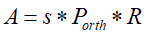
定义和计算A、pc和b:
- 定义A:
A = s*P.dot(R)
- 计算pc:
这里的pc计算相当于下式
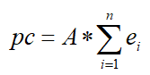
将表情主成分expPC转换为(29,68,3)的新矩阵pc_3d
pc_3d = np.resize(expPC.T, [dof, n, 3])
注意:这里的expPC经过了
expPC = model['expPC'][valid_ind, :n_ep]
运算,只包含特征点的表情主成分,格式为(683,29)
将pc_3d转换为(2968,3)的格式:
pc_3d = np.reshape(pc_3d, [dof*n, 3])
计算出
p
c
2
d
=
p
c
3
d
⋅
A
T
pc_{2d}= pc_{3d}\cdot A^T
pc2d=pc3d⋅AT,pc_2d格式为(29*68,2):
pc_2d = pc_3d.dot(A.T)
得出将pc_2d展开后得pc:
pc = np.reshape(pc_2d, [dof, -1]).T
- 定义b
b的公式如下:
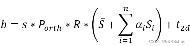
计算时由于矩阵的格式问题要先进行一些变换:
这里的shapeMU也是只包含了68个特征点的
将格式为(68*3,1)的shapeMU转换为格式(3,68):
mu_3d = np.resize(shapeMU, [n, 3]).T
这里的shape = shapePC.dot(sp),即 ∑ i = 1 m a i S i \sum_{i=1}^{m}a_iS_i ∑i=1maiSi:
shape_3d = shape
到这里b就可以按照公式计算出来了,得到的b格式为(2,68)
b = A.dot(mu_3d + shape_3d) + np.tile(t2d[:, np.newaxis], [1, n])
然后将b转换为格式(68*2,1)
b = np.reshape(b.T, [-1, 1])
求取β
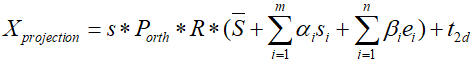
完成A、pc和b的定义和计算之后
X
p
r
o
j
e
c
t
i
o
n
X_{projection}
Xprojection 的公式就可以写成:
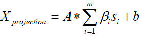
带入pc的式子可以写成:
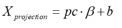
将
X
p
r
o
j
e
c
t
i
o
n
X_{projection}
Xprojection 的公式带入能量方程:
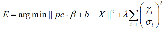
得到对β 进行求导,得到导数为零时β 的取值。
L2范数求导可以使用公式:
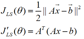
得到:
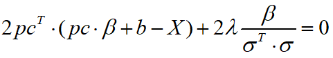
化简得到:
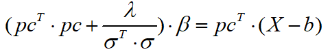
接着就是求取β 的代码:
equation_left = np.dot(pc.T, pc) + lamb * np.diagflat(1/sigma**2)
x = np.reshape(x.T, [-1, 1])
equation_right = np.dot(pc.T, x - b)
exp_para = np.dot(np.linalg.inv(equation_left), equation_right)
1.2 (4).将(2)和(3)中求出的β代入能量方程,解得α
同理,求取α 的代码如下:
expression = expPC.dot(ep)
expression = np.reshape(expression, [int(len(expression)/3), 3]).T
sp = estimate_shape(x, shapeMU, shapePC, model['shapeEV'][:n_sp,:], expression, s, R, t[:2], lamb = 0.004)
算法过程与求取β 相同,但是带入的β 是经过上面计算后的新值。
1.3 (5)更新α , β 的值,重复(2)-(4)进行迭代更新
到这里,循环迭代部分的代码告一段落,经过多次迭代计算(程序中给的迭代次数为三次),获得了所需要的sp, ep, s, R, t。
回到例程
回到bfm.fit从
fitted_sp, fitted_ep, s, R, t = fit.fit_points(x, X_ind, self.model, n_sp = self.n_shape_para, n_ep = self.n_exp_para, max_iter = max_iter)
继续向下执行:
def fit(self, x, X_ind, max_iter = 4, isShow = False):
        ''' fit 3dmm & pose parameters
        Args:
            x: (n, 2) image points
            X_ind: (n,) corresponding Model vertex indices
            max_iter: iteration
            isShow: whether to reserve middle results for show
        Returns:
            fitted_sp: (n_sp, 1). shape parameters
            fitted_ep: (n_ep, 1). exp parameters
            s, angles, t
        '''
        if isShow:
            fitted_sp, fitted_ep, s, R, t = fit.fit_points_for_show(x, X_ind, self.model, n_sp = self.n_shape_para, n_ep = self.n_exp_para, max_iter = max_iter)
            angles = np.zeros((R.shape[0], 3))
            for i in range(R.shape[0]):
                angles[i] = mesh.transform.matrix2angle(R[i])
        else:
            fitted_sp, fitted_ep, s, R, t = fit.fit_points(x, X_ind, self.model, n_sp = self.n_shape_para, n_ep = self.n_exp_para, max_iter = max_iter)
            angles = mesh.transform.matrix2angle(R)
        return fitted_sp, fitted_ep, s, angles, t
将旋转矩阵转换为XYZ角度angles = mesh.transform.matrix2angle(R)
之后返回fitted_sp, fitted_ep, s, angles, t。
回到3DMM例程
fitted_sp, fitted_ep, fitted_s, fitted_angles, fitted_t = bfm.fit(x, X_ind, max_iter = 3)
部分执行完毕,继续向下执行:
x = projected_vertices[bfm.kpt_ind, :2] # 2d keypoint, which can be detected from image
X_ind = bfm.kpt_ind # index of keypoints in 3DMM. fixed.

# fit
fitted_sp, fitted_ep, fitted_s, fitted_angles, fitted_t = bfm.fit(x, X_ind, max_iter = 3)

# verify fitted parameters
fitted_vertices = bfm.generate_vertices(fitted_sp, fitted_ep)
transformed_vertices = bfm.transform(fitted_vertices, fitted_s, fitted_angles, fitted_t)

image_vertices = mesh.transform.to_image(transformed_vertices, h, w)
fitted_image = mesh.render.render_colors(image_vertices, bfm.triangles, colors, h, w)
接下来是
fitted_vertices = bfm.generate_vertices(fitted_sp, fitted_ep)
根据计算出的α , β 代入
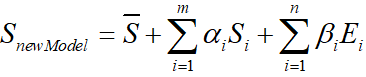
算出
S
n
e
w
M
o
d
e
l
S_{newModel}
SnewModel ,对应的源码如下:
 def generate_vertices(self, shape_para, exp_para):
        '''
        Args:
            shape_para: (n_shape_para, 1)
            exp_para: (n_exp_para, 1)
        Returns:
            vertices: (nver, 3)
        '''
        vertices = self.model['shapeMU'] + \
                   self.model['shapePC'].dot(shape_para) + \
                   self.model['expPC'].dot(exp_para)
        vertices = np.reshape(vertices, [int(3), int(len(vertices)/3)], 'F').T

        return vertices
算出
S
n
e
w
M
o
d
e
l
S_{newModel}
SnewModel 后再对三维模型进行相似变换:
transformed_vertices = bfm.transform(fitted_vertices, fitted_s, fitted_angles, fitted_t)
即 S t r a n f o r m e d = s ⋅ R ⋅ S n e w M o d e l + t 3 d S_{tranformed}=s\cdot R\cdot S_{newModel}+t_{3d} Stranformed=s⋅R⋅SnewModel+t3d
 def transform(self, vertices, s, angles, t3d):
        R = mesh.transform.angle2matrix(angles)
        return mesh.transform.similarity_transform(vertices, s, R, t3d)
之后的代码:
image_vertices = mesh.transform.to_image(transformed_vertices, h, w)
fitted_image = mesh.render.render_colors(image_vertices, bfm.triangles, colors, h, w)
分别是将三维模型转为二维图像的格式并用自带的颜色信息对模型上色,这里不做过多解读了。
结果展示
生成的新的人脸图片被保存到results/3dmm目录下
# ------------- print & show
print('pose, groudtruth: \n', s, angles[0], angles[1], angles[2], t[0], t[1])
print('pose, fitted: \n', fitted_s, fitted_angles[0], fitted_angles[1], fitted_angles[2], fitted_t[0], fitted_t[1])

save_folder = 'results/3dmm'
if not os.path.exists(save_folder):
    os.mkdir(save_folder)

io.imsave('{}/generated.jpg'.format(save_folder), image)
io.imsave('{}/fitted.jpg'.format(save_folder), fitted_image)
还可以通过生成一个gif展示特征点拟合的过程:
# fit

fitted_sp, fitted_ep, fitted_s, fitted_angles, fitted_t = bfm.fit(x, X_ind, max_iter = 3, isShow = True)

# verify fitted parameters
for i in range(fitted_sp.shape[0]):
	fitted_vertices = bfm.generate_vertices(fitted_sp[i], fitted_ep[i])
	transformed_vertices = bfm.transform(fitted_vertices, fitted_s[i], fitted_angles[i], fitted_t[i])

	image_vertices = mesh.transform.to_image(transformed_vertices, h, w)
	fitted_image = mesh.render.render_colors(image_vertices, bfm.triangles, colors, h, w)
	io.imsave('{}/show_{:0>2d}.jpg'.format(save_folder, i), fitted_image)

options = '-delay 20 -loop 0 -layers optimize' # gif. need ImageMagick.
subprocess.call('convert {} {}/show_*.jpg {}'.format(options, save_folder, save_folder + '/3dmm.gif'), shell=True)
subprocess.call('rm {}/show_*.jpg'.format(save_folder), shell=True)
下面是结果展示:
-
generated.jpg

-
fitted.jpg

-
3dmm.gif

当然,每次执行程序生成的新的随机模型的样子也会不同。
总结
这里主要介绍基于3DMM模型的反向过程求解α , β 的过程。很多细节还是要对照代码去理解公式与原理,结合公式去指导代码阅读。