目录
- 11神经网络demo1
- 12神经网络demo2
- 13神经网络demo3
- 20tensorflow2.0 安装教程,所有安装工具(神经网络)
- 21神经网络-线性回归- demo1
- 22神经网络-线性回归- demo2
- 28神经网络-多层感知- demo1
- 目录
11神经网络demo1
package com.example.xxx;
import java.util.Vector;

class Data
{
    Vector<Double> x = new Vector<Double>();       //输入数据
    Vector<Double> y = new Vector<Double>();       //输出数据
};

 class BPNN {

    final int LAYER = 3;        //三层神经网络
    final int NUM = 10;       //每层的最多节点数

    float A = (float) 30.0;
    float B = (float) 10.0;     //A和B是S型函数的参数
    int ITERS = 1000;     //最大训练次数
    float ETA_W = (float) 0.0035;   //权值调整率
    float ETA_B = (float) 0.001;    //阀值调整率
    float ERROR = (float) 0.002;    //单个样本允许的误差
    float ACCU = (float) 0.005;    //每次迭代允许的误差


    int in_num;                 //输入层节点数
    int ou_num;                 //输出层节点数
    int hd_num;                 //隐含层节点数

    Double[][][] w =new Double[LAYER][NUM][NUM];    //BP网络的权值
    Double[][] b = new Double[LAYER][NUM];         //BP网络节点的阀值

    Double[][] x= new Double[LAYER][NUM];         //每个神经元的值经S型函数转化后的输出值,输入层就为原值
    Double[][] d= new Double[LAYER][NUM];         //记录delta学习规则中delta的值


    Vector<Data> data;

    //获取训练所有样本数据
    void GetData(Vector<Data> _data) {
        data = _data;
    }
    //开始进行训练
    void Train() {
        System.out.printf("Begin to train BP NetWork!\n");
        GetNums();
        InitNetWork();
        int num = data.size();

        for(int iter = 0; iter <= ITERS; iter++) {
            for(int cnt = 0; cnt < num; cnt++) {
                //第一层输入节点赋值
                for(int i = 0; i < in_num; i++)
                    x[0][i] = data.get(cnt).x.get(i);

                while(true)
                {
                    ForwardTransfer();
                    if(GetError(cnt) < ERROR)    //如果误差比较小,则针对单个样本跳出循环
                        break;
                    ReverseTransfer(cnt);
                }
            }
            System.out.printf("This is the %d th trainning NetWork !\n", iter);

            Double accu = GetAccu();
            System.out.printf("All Samples Accuracy is " + accu);
            if(accu < ACCU) break;
        }
        System.out.printf("The BP NetWork train End!\n");
    }

    //根据训练好的网络来预测输出值
    Vector<Double> ForeCast(Vector<Double> data) {
        int n = data.size();
        assert(n == in_num);
        for(int i = 0; i < in_num; i++)
            x[0][i] = data.get(i);

        ForwardTransfer();
        Vector<Double> v = new Vector<Double>();
        for(int i = 0; i < ou_num; i++)
            v.add(x[2][i]);
        return v;
    }

    //获取网络节点数
    void GetNums() {
        in_num = data.get(0).x.size();                         //获取输入层节点数
        ou_num = data.get(0).y.size();                         //获取输出层节点数
        hd_num = (int)Math.sqrt((in_num + ou_num) * 1.0) + 5;   //获取隐含层节点数
        if(hd_num > NUM) hd_num = NUM;                     //隐含层数目不能超过最大设置
    }

    //初始化网络
    void InitNetWork() {
        for(int i = 0; i < LAYER; i++){
            for(int j = 0; j < NUM; j++){
                for(int k = 0; k < NUM; k++){
                    w[i][j][k] = 0.0;
                }
            }
        }
        for(int i = 0; i < LAYER; i++){
            for(int j = 0; j < NUM; j++){
                b[i][j] = 0.0;
            }
        }
    }

    //工作信号正向传递子过程
    void ForwardTransfer() {
        //计算隐含层各个节点的输出值
        for(int j = 0; j < hd_num; j++) {
            Double t = 0.0;
            for(int i = 0; i < in_num; i++)
                t += w[1][i][j] * x[0][i];
            t += b[1][j];
            x[1][j] = Sigmoid(t);
        }

        //计算输出层各节点的输出值
        for(int j = 0; j < ou_num; j++) {
            Double t = (double) 0;
            for(int i = 0; i < hd_num; i++)
                t += w[2][i][j] * x[1][i];
            t += b[2][j];
            x[2][j] = Sigmoid(t);
        }
    }

    //计算单个样本的误差
    double GetError(int cnt) {
        Double ans = (double) 0;
        for(int i = 0; i < ou_num; i++)
            ans += 0.5 * (x[2][i] - data.get(cnt).y.get(i)) * (x[2][i] - data.get(cnt).y.get(i));
        return ans;
    }

    //误差信号反向传递子过程
    void ReverseTransfer(int cnt) {
        CalcDelta(cnt);
        UpdateNetWork();
    }

    //计算所有样本的精度
    double GetAccu() {
        Double ans = (double) 0;
        int num = data.size();
        for(int i = 0; i < num; i++) {
            int m = data.get(i).x.size();
            for(int j = 0; j < m; j++)
                x[0][j] = data.get(i).x.get(j);
            ForwardTransfer();
            int n = data.get(i).y.size();
            for(int j = 0; j < n; j++)
                ans += 0.5 * (x[2][j] - data.get(i).y.get(j)) * (x[2][j] - data.get(i).y.get(j));
        }
        return ans / num;
    }

    //计算调整量
    void CalcDelta(int cnt) {
        //计算输出层的delta值
        for(int i = 0; i < ou_num; i++)
            d[2][i] = (x[2][i] - data.get(cnt).y.get(i)) * x[2][i] * (A - x[2][i]) / (A * B);
        //计算隐含层的delta值
        for(int i = 0; i < hd_num; i++) {
            Double t = (double) 0;
            for(int j = 0; j < ou_num; j++)
                t += w[2][i][j] * d[2][j];
            d[1][i] = t * x[1][i] * (A - x[1][i]) / (A * B);
        }
    }

    //根据计算出的调整量对BP网络进行调整
    void UpdateNetWork() {
        //隐含层和输出层之间权值和阀值调整
        for(int i = 0; i < hd_num; i++) {
            for(int j = 0; j < ou_num; j++)
                w[2][i][j] -= ETA_W * d[2][j] * x[1][i];
        }
        for(int i = 0; i < ou_num; i++)
            b[2][i] -= ETA_B * d[2][i];

        //输入层和隐含层之间权值和阀值调整
        for(int i = 0; i < in_num; i++) {
            for(int j = 0; j < hd_num; j++)
                w[1][i][j] -= ETA_W * d[1][j] * x[0][i];
        }
        for(int i = 0; i < hd_num; i++)
            b[1][i] -= ETA_B * d[1][i];
    }

    //计算Sigmoid函数的值
    Double Sigmoid(double x) {
        return A / (1 + Math.exp(-x / B));
    }

}
package com.example.xxx;

import java.io.IOException;
import java.util.Vector;

public class xxx2 {

}


class BPNeuralNetworks {

    static Double[][] sample=
            {
                    {0.0,0.0,0.0,0.0},
                    {5.0,1.0,4.0,19.020},
                    {5.0,3.0,3.0,14.150},
                    {5.0,5.0,2.0,14.360},
                    {5.0,3.0,3.0,14.150},
                    {5.0,3.0,2.0,15.390},
                    {5.0,3.0,2.0,15.390},
                    {5.0,5.0,1.0,19.680},
                    {5.0,1.0,2.0,21.060},
                    {5.0,3.0,3.0,14.150},
                    {5.0,5.0,4.0,12.680},
                    {5.0,5.0,2.0,14.360},
                    {5.0,1.0,3.0,19.610},
                    {5.0,3.0,4.0,13.650},
                    {5.0,5.0,5.0,12.430},
                    {5.0,1.0,4.0,19.020},
                    {5.0,1.0,4.0,19.020},
                    {5.0,3.0,5.0,13.390},
                    {5.0,5.0,4.0,12.680},
                    {5.0,1.0,3.0,19.610},
                    {5.0,3.0,2.0,15.390},
                    {1.0,3.0,1.0,11.110},
                    {1.0,5.0,2.0,6.521},
                    {1.0,1.0,3.0,10.190},
                    {1.0,3.0,4.0,6.043},
                    {1.0,5.0,5.0,5.242},
                    {1.0,5.0,3.0,5.724},
                    {1.0,1.0,4.0,9.766},
                    {1.0,3.0,5.0,5.870},
                    {1.0,5.0,4.0,5.406},
                    {1.0,1.0,3.0,10.190},
                    {1.0,1.0,5.0,9.545},
                    {1.0,3.0,4.0,6.043},
                    {1.0,5.0,3.0,5.724},
                    {1.0,1.0,2.0,11.250},
                    {1.0,3.0,1.0,11.110},
                    {1.0,3.0,3.0,6.380},
                    {1.0,5.0,2.0,6.521},
                    {1.0,1.0,1.0,16.000},
                    {1.0,3.0,2.0,7.219},
                    {1.0,5.0,3.0,5.724}
            };

    public static void main( String[] args ) throws IOException
    {
        Vector<Data> data = new Vector<Data>();
        System.out.println("===>"+sample.length);
        for(int i = 0; i < sample.length; i++)
        {
            Data t = new Data();
            for(int j = 0; j < 3; j++)
                t.x.add(sample[i][j]);
            t.y.add(sample[i][3]);
            data.add(t);
        }
        BPNN bp = new BPNN();
        bp.GetData(data);
        bp.Train();

        while(true)
        {
            Vector<Double> in = new Vector<Double>();
            for(int i = 0; i < 3; i++)
            {
                Double v = 0.0;
                in.add(v);
            }
            Vector<Double> ou;
            ou = bp.ForeCast(in);
            System.out.println("===>   "+ou.get(0));
        }
    }

}
···················································································································································································
12神经网络demo2
package com.example.xxx;
import java.util.ArrayList;
import java.util.List;
import java.util.Random;
public class xxxx {
}

class Neuron {

    /**
     * 神经元值
     */
    public double value;
    /**
     * 神经元输出值
     */
    public double o;

    public Neuron () {
        init ();
    }
    public Neuron (double v) {
        init (v);
    }
    public Neuron (double v, double o) {
        this.value = v;
        this.o = o;
    }

    public void init () {
        this.value = 0;
        this.o = 0;
    }
    public void init (double v) {
        this.value = v;
        this.o = 0;
    }
    public void init (double v, double o) {
        this.value = v;
        this.o = o;
    }

    /**
     * sigmod激活函数
     */
    public void sigmod () {
        this.o = 1.0 / ( 1.0 + Math.exp(-1.0 * this.value));
    }

    public String toString () {
        return "(" + value + " " + o + ")";
    }
}


class RandomUtil {
    public static final int RAND_SEED = 2016;
    public static Random rand = new Random (RAND_SEED);

    public static double nextDouble () {
        return rand.nextDouble();
    }
    public static double nextDouble (double a, double b) {
        if (a > b) {
            double tmp = a;
            a = b;
            b = tmp;
        }
        return rand.nextDouble() * (b - a) + a;
    }
}


class NeuronNet {
    /**
     * 神经网络
     */
    public List<List<Neuron>> neurons;
    /**
     * 网络权重, weight[i][j][k] = 第i层和第i+1层之间, j神经元和k神经元的权重, i = 0 ... layer-1
     */
    public double [][][] weight;
    /**
     * 下一层网络残差, deta[i][j] = 第i层, 第j神经元的残差, i = 1 ... layer-1
     */
    public double [][] deta;

    /**
     * 网络层数(包括输入与输出层)
     */
    public int layer;
    /**
     * 学习率
     */
    public static final double RATE = 0.1;
    /**
     * 误差停止阈值
     */
    public static final double STOP = 0.0001;
    /**
     * 迭代次数阈值
     */
    public static final int NUMBER_ROUND = 5000000;

    public NeuronNet () {

    }
    public NeuronNet (int [] lens) {
        init (lens);
    }

    public void init (int [] lens) {
        layer = lens.length;
        neurons = new ArrayList<List<Neuron>>();

        for (int i = 0; i < layer; ++ i) {
            List<Neuron> list = new ArrayList<Neuron> ();
            for (int j = 0; j < lens[i]; ++ j) {
                list.add(new Neuron ());
            }
            neurons.add(list);
        }

        weight = new double [layer-1][][];
        for (int i = 0; i < layer-1; ++ i) {
            weight[i] = new double [lens[i]][];
            for (int j = 0; j < lens[i]; ++ j) {
                weight[i][j] = new double [lens[i+1]];
                for (int k = 0; k < lens[i+1]; ++ k) {
                    weight[i][j][k] = RandomUtil.nextDouble(0, 0.1);
                }
            }
        }

        deta = new double [layer][];
        for (int i = 0; i < layer; ++ i) {
            deta[i] = new double [lens[i]];
            for (int j = 0; j < lens[i]; ++ j) deta[i][j] = 0;
        }
    }

    /**
     * 前向传播
     * @param features
     * @return
     */
    public boolean forward (double [] features) {
        // c = layer index
        for (int c = 0; c < layer; ++ c) {
            if (c == 0) {
                // 初始化输入层

                List<Neuron> inputLayer = neurons.get(c);
                if (inputLayer.size() != features.length) {
                    System.err.println("[error] Feature length != input layer neuron number");
                    return false;
                }
                for (int i = 0; i < inputLayer.size(); ++ i) {
                    Neuron neuron = inputLayer.get(i);
                    neuron.init(features[i], features[i]);
                }
            } else {
                // 前向传播:从c-1层传播到c层
                List<Neuron> vList = neurons.get(c);
                List<Neuron> uList = neurons.get(c-1);
                for (int i = 0; i < vList.size(); ++ i) {
                    Neuron v = vList.get(i);
                    v.value = 0;
                    for (int j = 0; j < uList.size(); ++ j) {
                        Neuron u = uList.get(j);
                        v.value += u.o * weight[c-1][j][i];
                    }
                    v.sigmod();
                }
            }
        }
        return true;
    }

    /**
     * 求误差函数
     * @param labels 期望输出层向量
     * @return
     */
    public double getError (double [] labels) {
        if (labels.length != neurons.get(layer-1).size()) {
            System.err.println("[error] label length != output layer neuron number");
            return -1;
        }
        double e = 0;
        for (int i = 0; i < labels.length; ++ i) {
            double o = neurons.get(layer-1).get(i).o;
            e += (labels[i] - o) * (labels[i] - o);
        }
        return e / 2;
    }
    /**
     * 获取输出层向量
     * @return
     */
    public double[] getOutput () {
        double [] output = new double [neurons.get(layer-1).size()];
        for (int i = output.length-1; i >= 0 ; -- i)
            output [i] = neurons.get(layer-1).get(i).o;
        return output;
    }

    /**
     * 反向传播
     * @param labels
     * @return
     */
    public boolean backward (double [] labels) {
        if (labels.length != neurons.get(layer-1).size()) {
            System.err.println("[error] label length != output layer neuron number");
            return false;
        }
        // 初始化output层(layer-1)残差
        for (int j = neurons.get(layer-1).size()-1; j >= 0 ; -- j) {
            double o = neurons.get(layer-1).get(j).o;
            // 求导公式
            deta[layer-1][j] = -1 * (labels[j] - o) * o * (1 - o);
            // 更新倒数第二层和最后一层之间的权重
            for (int i = neurons.get(layer-2).size()-1; i >= 0; -- i) {
                weight[layer-2][i][j] -= RATE * deta[layer-1][j] * neurons.get(layer-2).get(i).o;
            }
        }
        //A层(layer=L)和B层(layer=L+1)间权重调整,用到了C层(layer=L+2)
        for (int l = layer-3; l >= 0; -- l) {

            // 遍历B层
            for (int j = neurons.get(l+1).size()-1; j >= 0; -- j) {
                // B层J神经元残差
                deta[l+1][j] = 0;
                // 遍历C层, 求残差和
                for (int k = neurons.get(l+2).size()-1; k >= 0; -- k) {
                    // C层残差通过权重weight传递过来
                    deta[l+1][j] += deta[l+2][k] * weight[l+1][j][k];
                }
                double o = neurons.get(l+1).get(j).o;
                deta[l+1][j] *= o * (1 - o);

                // 遍历A层
                for (int i = neurons.get(l).size()-1; i >= 0; -- i) {
                    // A层i神经元和B层j神经元权重
                    weight[l][i][j] -= RATE * deta[l+1][j] * neurons.get(l).get(i).o;
                }
            }
        }
        return true;
    }

    public void train (double [][] features, double [][] labels) {
        SGD (features, labels);
    }

    public void SGD (double [][] features, double [][] labels) {
        int num = 0;
        double error = 1;
        while ((num ++) <= NUMBER_ROUND && error > STOP) {
            for (int i = 0; i < features.length; ++ i) {
                boolean flag = forward (features[i]);
                if (!flag) {
                    return;
                }

                error = this.getError(labels[i]);
                if (error == -1) {
                    return;
                }

                if (error <= STOP)
                    break;

                flag = backward (labels[i]);
                if (!flag) {
                    return;
                }
            }
            System.out.println("[Info] Times = " + num + ", error = " + error);
        }
    }

    public double [] predict (double [] feature) {
        forward (feature);
        return this.getOutput();
    }
}


class Main {
    public static void main(String[] args) {
        // 三层神经网络,每层神经元个数分别是3,5,8
        NeuronNet bpnn = new NeuronNet (new int [] {3, 5, 8});

        // 数据说明,求二进制X[i]的十进制表示Y[i]
        double[][] X = {
                {0,0,0},
                {0,0,1},
                {0,1,0},
                {0,1,1},
                {1,0,0},
                {1,0,1},
                {1,1,0},
                {1,1,1}
        };
        double [][] Y = {
                {1, 0, 0, 0, 0, 0, 0, 0},
                {0, 1, 0, 0, 0, 0, 0, 0},
                {0, 0, 1, 0, 0, 0, 0, 0},
                {0, 0, 0, 1, 0, 0, 0, 0},
                {0, 0, 0, 0, 1, 0, 0, 0},
                {0, 0, 0, 0, 0, 1, 0, 0},
                {0, 0, 0, 0, 0, 0, 1, 0},
                {0, 0, 0, 0, 0, 0, 0, 1}
        };

        bpnn.train(X, Y);

        for (int i = 0; i < 8; ++ i) {
            double [] output = bpnn.predict(X[i]);
            double max = -1;
            int pos = -1;
            // 求最接近的神经元
            for (int j = 0; j < output.length; ++ j) {
                if (max < output[j]) {
                    max = output[j];
                    pos = j;
                }
            }
            System.out.print (X[i][0]);
            for (int j = 1; j < X[i].length; ++ j) {
                System.out.print (", " + X[i][j]);
            }
            System.out.println(" = " + pos);
        }
    }
}
···················································································································································································
13神经网络demo3
package com.example.xxx;

import java.io.BufferedReader;
import java.io.File;
import java.io.FileInputStream;
import java.io.InputStreamReader;
import java.util.ArrayList;

public class xxxx {

}

class Main {
    private static String path = "./src/data.txt";  //deta数据在最下面
    private static ArrayList<ArrayList<String>> data = new ArrayList<ArrayList<String>>();

    public static void main(String[] args) {
        readData(path);
        //对缺失值进行处理,但文件data.txt不处理,可能对缺失值进行另一种方法处理
         //山鸢尾,变色鸢尾, 和维吉尼亚鸢尾, 分类3种花 (包括决策树、贝叶斯分类方法、BP神经网络和SVM)
        dealWithData();
        System.out.println("对数据进行朴素贝叶斯分类:");
        Bayesian bayesian = new Bayesian("6.4","2.7","5.3","1.8",data);
        bayesian.calculate_Bayesian();
        Bayesian bayesian1 = new Bayesian("4.5","2.3", "1.3", "0.3",data);
        bayesian1.calculate_Bayesian();
        Bayesian bayesian2 = new Bayesian("5.5","2.6","4.4","1.2",data);
        bayesian2.calculate_Bayesian();
        Bayesian bayesian3 = new Bayesian("5.1","2.5","3.0","1.1",data);
        bayesian3.calculate_Bayesian();
        Bayesian bayesian4 = new Bayesian("6.7","3.0","5.0","1.7",data);
        bayesian4.calculate_Bayesian();
        //show();
    }

    /**
     * -1代表缺失值,通过计算属性的平均值作为缺失值的填补值。
     */
    private static void dealWithData() {
        double sum1 = 0.0, sum2 = 0.0, sum3 = 0.0, sum4 = 0.0;
        double value1, value2, value3, value4;
        int len1 = data.size(),len2 = data.size(),len3 = data.size(),len4 = data.size();
        for (int i=0; i<data.size(); i++){
            if (!data.get(i).get(0).equals("-1")){
                sum1 += Double.parseDouble(data.get(i).get(0));
                len1--;
            }
            if (!data.get(i).get(1).equals("-1")){
                sum2 += Double.parseDouble(data.get(i).get(1));
                len2--;
            }
            if (!data.get(i).get(2).equals("-1")){
                sum3 += Double.parseDouble(data.get(i).get(2));
                len3--;
            }
            if (!data.get(i).get(3).equals("-1")){
                sum4 += Double.parseDouble(data.get(i).get(3));
                len4--;
            }
        }
        value1 = sum1/(len1*1.0);
        value2 = sum2/(len2*1.0);
        value3 = sum3/(len3*1.0);
        value4 = sum4/(len4 *1.0);
        for (int j=0; j<data.size(); j++){
            if (data.get(j).get(0).equals("-1")){
                data.get(j).set(0,Double.toString(value1));
            }
            if (data.get(j).get(1).equals("-1")){
                data.get(j).set(1,Double.toString(value2));
            }
            if (data.get(j).get(2).equals("-1")){
                data.get(j).set(2,Double.toString(value3));
            }
            if (data.get(j).get(3).equals("-1")){
                data.get(j).set(3,Double.toString(value4));
            }
        }
    }


    /**
     * 导入数据到data
     * @param path
     * @return
     */
    public  static ArrayList<ArrayList<String>> readData(String path){
        ArrayList<String> d = null;
        ArrayList<ArrayList<String>> t = new ArrayList<ArrayList<String>>();

        try {
            InputStreamReader isr = new InputStreamReader(new FileInputStream(new File(path)));
            BufferedReader br = new BufferedReader(isr);
            String str = null;
            while((str = br.readLine()) != null){
                d = new ArrayList<String>();
                String[] str1 = str.split(",");
                for(int i = 0; i < str1.length ; i++) {
                    d.add(str1[i]);
                }
                t.add(d);
            }
            data = t;
            br.close();
            isr.close();
        } catch (Exception e) {
            e.printStackTrace();
            System.out.println("读取文件内容出错!");
        }
        return t;
    }

    /**
     * 遍历data
     */
    public static void show(){
        for(int i=0;i<data.size();i++){
            System.out.println(data.get(i));
        }
    }

}

class Bayesian {
    private String calyx_len;
    private String calyx_wid;
    private String petal_len;
    private String petal_wid;
    private ArrayList<ArrayList<String>> data;
    public Bayesian(String calyx_len, String calyx_wid, String petal_len, String petal_wid, ArrayList<ArrayList<String>> data){
        this.calyx_len = calyx_len;
        this.calyx_wid = calyx_wid;
        this.petal_len = petal_len;
        this.petal_wid = petal_wid;
        this.data = data;
    }

    /**
     * 贝叶斯运算部分
     */
    public void calculate_Bayesian(){
        //获取P(Iris-setosa|Iris-versicolor|Iris-virginica)的分子————————————P(x|y)的分母
        int setosa = getNums("Iris-setosa");
        int versicolor = getNums("Iris-versicolor");
        int virginica = getNums("Iris-virginica");
        /**
         * 对数据进行划分等级,取整数位为分级标准
         * 花萼长度以4.x,5.x,6.x,7.x为等级
         * 花萼宽度以2.x,3.x,4.x
         * 花瓣长度以1.x,3.x,4.x,5.x,6.x
         * 花瓣宽度以0.x,1.x,2.x
         */
        //获取P(x|y)的分子,0代表花萼长度,1代表花萼宽度,2代表花瓣长度,3代表花瓣宽度
        int calyx_len_setosa = getNums(0,calyx_len,"Iris-setosa");
        int calyx_wid_setosa = getNums(1,calyx_wid,"Iris-setosa");
        int petal_len_setosa = getNums(2,petal_len,"Iris-setosa");
        int petal_wid_setosa = getNums(3,petal_wid,"Iris-setosa");
        int calyx_len_versicolor = getNums(0,calyx_len,"Iris-versicolor");
        int calyx_wid_versicolor = getNums(1,calyx_wid,"Iris-versicolor");
        int petal_len_versicolor = getNums(2,petal_len,"Iris-versicolor");
        int petal_wid_versicolor = getNums(3,petal_wid,"Iris-versicolor");
        int calyx_len_virginica = getNums(0,calyx_len,"Iris-virginica");
        int calyx_wid_virginica = getNums(1,calyx_wid,"Iris-virginica");
        int petal_len_virginica = getNums(2,petal_len,"Iris-virginica");
        int petal_wid_virginica = getNums(3,petal_wid,"Iris-virginica");

        //计算概率Iris_setosa,Iris_versicolor,Iris_virginica
        double setosa_probability = (setosa/(data.size()*1.0))*(calyx_len_setosa/(setosa*1.0))
                *(calyx_wid_setosa/(setosa*1.0))*(petal_len_setosa/(setosa*1.0))*(petal_wid_setosa/(setosa*1.0));
        double versicolor_probability = (versicolor/(data.size()*1.0))*(calyx_len_versicolor/(versicolor*1.0))
                *(calyx_wid_versicolor/(versicolor*1.0))*(petal_len_versicolor/(versicolor*1.0))*(petal_wid_versicolor/(versicolor*1.0));
        double virginica_probability = (virginica/(data.size()*1.0))*(calyx_len_virginica/(virginica*1.0))
                *(calyx_wid_virginica/(virginica*1.0))*(petal_len_virginica/(virginica*1.0))*(petal_wid_virginica/(virginica*1.0));


        //比较概率得出结论
        if(setosa_probability > versicolor_probability && setosa_probability > virginica_probability){
            System.out.println("<"+calyx_len+","+calyx_wid+","+petal_len+","+petal_wid+","+">  ---> Iris-setosa");
        }
        if(versicolor_probability > setosa_probability && versicolor_probability > virginica_probability){
            System.out.println("<"+calyx_len+","+calyx_wid+","+petal_len+","+petal_wid+","+">  ---> Iris-versicolor");
        }
        if(virginica_probability > setosa_probability && virginica_probability > versicolor_probability){
            System.out.println("<"+calyx_len+","+calyx_wid+","+petal_len+","+petal_wid+","+">  ---> Iris-virginica");
        }
    }


    private int getNums(String str) {
        int num = 0;
        for(int i=0;i<data.size();i++){
            if(data.get(i).get(4).equals(str)){
                num++;
            }
        }
        return num;
    }
    private int getNums(int id, String str1, String str2){
        int num = 0;
        for(int i=0;i<data.size();i++){
            if(data.get(i).get(4).equals(str2)){
                if(data.get(i).get(id).charAt(0) == str1.charAt(0)){
                    num++;
                }
            }
        }
        return num;
    }
}


        // 5.1,3.5,1.4,0.2,Iris-setosa
        // -1,3.0,1.4,0.2,Iris-setosa
        // 4.7,3.2,1.3,0.2,Iris-setosa
        // 4.6,3.1,-1,0.2,Iris-setosa
        // 5.0,3.6,1.4,0.2,Iris-setosa
        // 5.5,2.3,4.0,1.3,Iris-versicolor
        // 6.5,2.8,4.6,1.5,Iris-versicolor
        // -1,2.8,4.5,1.3,Iris-versicolor
        // 6.3,3.3,4.7,1.6,Iris-versicolor
        // 7.1,3.0,5.9,2.1,Iris-virginica
        // -1,2.9,5.6,1.8,Iris-virginica
        // 6.5,3.0,5.8,2.2,Iris-virginica
        // 4.9,2.4,3.3,1.0,Iris-versicolor
        // 5.6,3.0,4.5,1.5,Iris-versicolor
        // 5.8,2.7,4.1,1.0,Iris-versicolor
        // 6.3,3.3,-1,2.5,Iris-virginica
        // 5.8,2.7,5.1,1.9,Iris-virginica
        // 7.6,3.0,6.6,2.1,Iris-virginica
        // 4.9,2.5,4.5,1.7,Iris-virginica
        // 7.3,2.9,6.3,1.8,Iris-virginica
        // 5.7,2.5,-1,2.0,Iris-virginica
        // 5.8,2.8,5.1,2.4,Iris-virginica
        // 6.6,2.9,4.6,1.3,Iris-versicolor
        // 5.2,2.7,3.9,1.4,Iris-versicolor
        // 5.4,3.9,1.7,0.4,Iris-setosa
        // 4.6,3.4,1.4,0.3,Iris-setosa
        // 5.0,3.4,1.5,0.2,Iris-setosa
        // 4.4,2.9,1.4,-1,Iris-setosa
        // 4.9,3.1,1.5,0.1,Iris-setosa
        // 5.4,3.7,1.5,0.2,Iris-setosa
        // 4.8,-1,1.6,0.2,Iris-setosa
        // 4.8,3.0,1.4,0.1,Iris-setosa
        // 4.3,3.0,1.1,0.1,Iris-setosa
        // 5.8,4.0,1.2,0.2,Iris-setosa
        // 6.1,2.9,4.7,1.4,Iris-versicolor
        // 5.6,2.9,3.6,1.3,Iris-versicolor
        // 6.7,3.1,4.4,1.4,Iris-versicolor
        // 6.4,3.2,5.3,2.3,Iris-virginica
        // 6.5,3.0,5.5,1.8,Iris-virginica
        // 5.7,4.4,1.5,0.4,Iris-setosa
        // 5.4,3.9,1.3,0.4,Iris-setosa
        // 5.1,3.5,1.4,0.3,Iris-setosa
        // 5.7,3.8,1.7,0.3,Iris-setosa
        // 5.1,3.8,-1,0.3,Iris-setosa
        // 5.4,3.4,1.7,0.2,Iris-setosa
        // 5.1,3.7,1.5,0.4,Iris-setosa
        // 6.7,2.5,5.8,-1,Iris-virginica
        // 7.2,3.6,6.1,2.5,Iris-virginica
        // 6.5,3.2,5.1,2.0,Iris-virginica
        // 6.8,3.0,5.5,2.1,Iris-virginica
        // 4.6,3.6,1.0,0.2,Iris-setosa
        // 5.1,3.3,1.7,0.5,Iris-setosa
        // -1,3.4,1.9,0.2,Iris-setosa
        // 5.0,3.0,1.6,0.2,Iris-setosa
        // 7.0,3.2,4.7,1.4,Iris-versicolor
        // 6.4,3.2,4.5,1.5,Iris-versicolor
        // 6.9,3.1,4.9,1.5,Iris-versicolor
        // 5.0,2.0,3.5,1.0,Iris-versicolor
        // 5.9,-1,4.2,1.5,Iris-versicolor
        // 6.0,2.2,4.0,1.0,Iris-versicolor
        // 7.7,3.8,6.7,2.2,Iris-virginica
        // 7.7,2.6,6.9,2.3,Iris-virginica
        // 6.0,2.2,5.0,-1,Iris-virginica
        // 6.9,3.2,5.7,2.3,Iris-virginica
···················································································································································································
20tensorflow2.0 安装教程,所有安装工具(神经网络)
安装:常用的工具 jupyter notebook
pip install tensorflow-cpu==2.3.0 -i https://pypi.douban.com/simple/
pip install seaborn -i https://pypi.douban.com/simple/
pip install matplotlib notebook -i https://pypi.douban.com/simple/

pip install sklearn -i https://pypi.douban.com/simple/
pip install xgboost -i https://pypi.douban.com/simple/
环境要求:
64位操作系统
ubuntu 16.04 或以上
windows 7 或以上
masOS 10.12.6 或以上
raspbian 9.0 或以上
python  3.5-3.7    ****版本升级,用更高版本***
搭建开发环境:
使用:miniconda   搭建环境
官网:https://docs.conda.io/en/latest/miniconda.html#windows-installers

它包括了:
1,conda包管理工具
2,python
windows用户需要安装VC
官网:http://support.microsoft.com/zh-cn/help/2977003/the-latest-supported-visual-c-downloads
安装完成 miniconda +  VC  环境安装就完毕。   安装完毕 需要重启电脑。 (下一步即可)
安装包在qq群里,也可以去官网下载,网站如上。

进入命令行查看版本如下
打开命令行窗口: Anaconda Prompt (tensorflow2.0)
输入查看命令: pip -V

安装tensorflow2…3.0版本
安装命令:(如下图) *版本升级,用更高版本
pip install tensorflow-cpu==2.3.0 -i https://pypi.douban.com/simple/

输入命令开始安装: (如下图)

安装完成 进行查看:
命令:如下
python
import tensorflow as tf
print(tf.__version__)
exit()
pip install matplotlib notebook -i https://pypi.douban.com/simple/

安装完成后 (matplotlib notebook)
进入notebook
jupyter notebook

→ 进入notebook → 弹窗如下 (自动弹窗)

导入tensorflow 查看版本
import tensorflow as tf
tf.version

···················································································································································································
21神经网络-线性回归- demo1
// Incomel.csv 为文件名 ./dataset/ 为路径
//进入
jupyter notebook
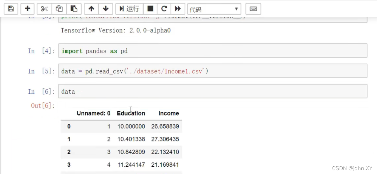
import pandas as pd
data = pd.read_csv('./dataset/Incomel.csv')
data
import matplotlib.pyplot as plt
%matplotlib inline
plt.scatter(data.Education,data.Income)
解释:
import pandas as pd 引入 → pandas
import matplotlib.pyplot as plt 为绘图工具 → 引入
%matplotlib inline 显示出来
plt.scatter(data.Education,data.Income) 绘制的文件的列名
Education,Income 为文件的列名
单变量线性回归算法方程式: f(x) = ax + b
下图为:引入文件
下图为:引入绘图工具

下图为:绘制的效果

···················································································································································································
22神经网络-线性回归- demo2
打开命令行窗口: Anaconda Prompt (tensorflow2.0)
进入notebook: jupyter notebook
1
import pathlib

import matplotlib.pyplot as plt
import pandas as pd
import seaborn as sns

import tensorflow as tf

from tensorflow import keras
from tensorflow.keras import layers

print(tf.__version__)
2 下载数据
dataset_path = keras.utils.get_file("auto-mpg.data", "http://archive.ics.uci.edu/ml/machine-learning-databases/auto-mpg/auto-mpg.data")
dataset_path
3 使用 pandas 导入数据集。
column_names = ['MPG','Cylinders','Displacement','Horsepower','Weight',
                'Acceleration', 'Model Year', 'Origin']
raw_dataset = pd.read_csv(dataset_path, names=column_names,
                      na_values = "?", comment='\t',
                      sep=" ", skipinitialspace=True)

dataset = raw_dataset.copy()
dataset.tail()
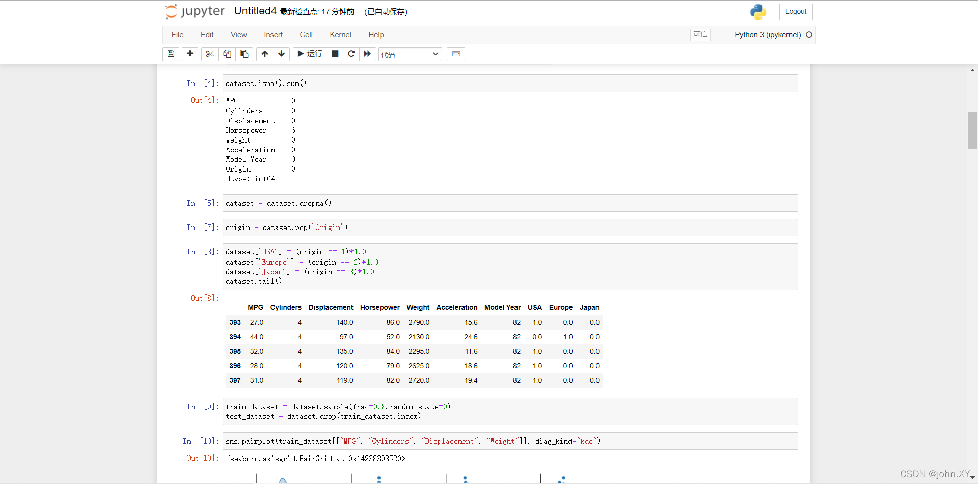
4 数据清洗,数据集中包括一些未知值。
dataset.isna().sum()
5 为了保证这个初始示例的简单性,删除这些行。
dataset = dataset.dropna()
7 (5 → 7) “Origin” 列实际上代表分类,而不仅仅是一个数字。所以把它转换为独热码 (one-hot)
origin = dataset.pop('Origin')
8
dataset['USA'] = (origin == 1)*1.0
dataset['Europe'] = (origin == 2)*1.0
dataset['Japan'] = (origin == 3)*1.0
dataset.tail()
9 拆分训练数据集和测试数据集,现在需要将数据集拆分为一个训练数据集和一个测试数据集,我们最后将使用测试数据集对模型进行评估。
train_dataset = dataset.sample(frac=0.8,random_state=0)
test_dataset = dataset.drop(train_dataset.index)
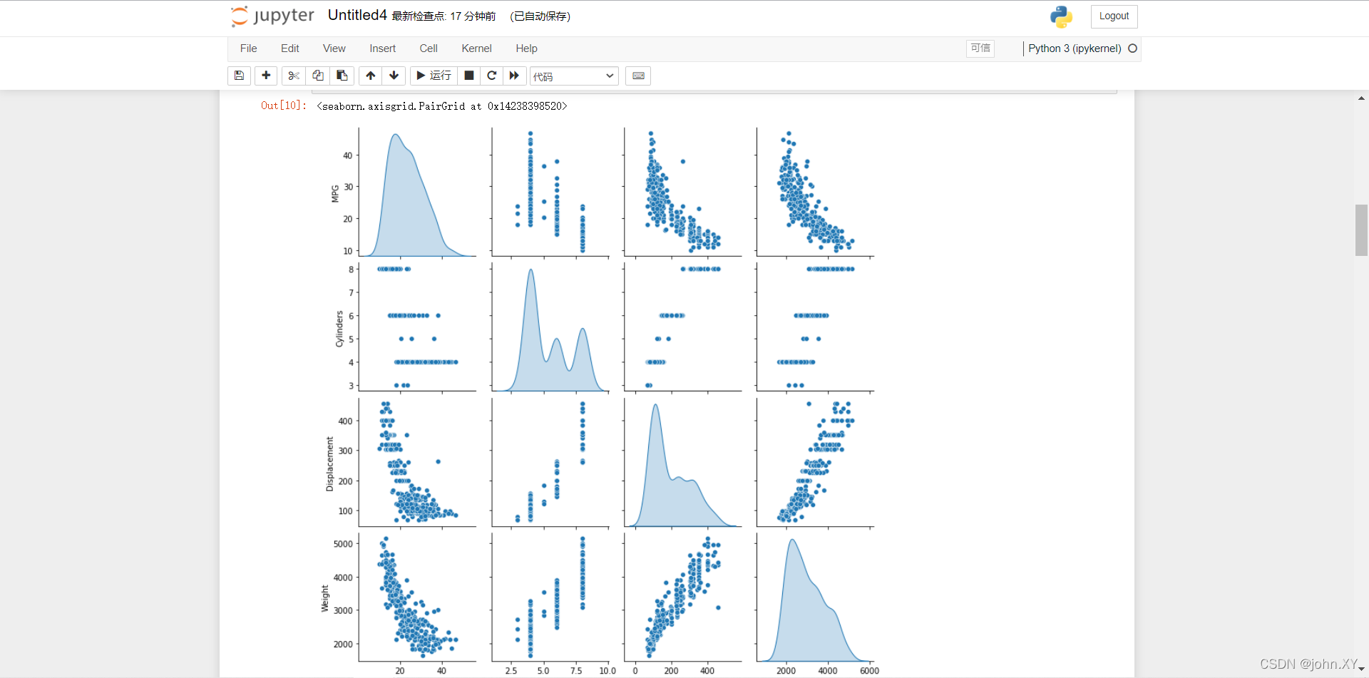
10 快速查看训练集中几对列的联合分布。
sns.pairplot(train_dataset[["MPG", "Cylinders", "Displacement", "Weight"]], diag_kind="kde")
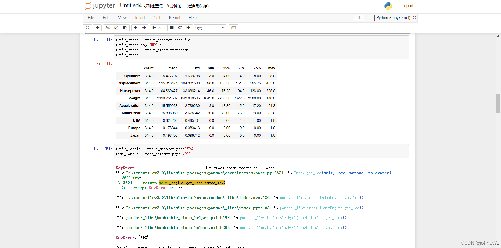
11 查看总体的数据统计。
train_stats = train_dataset.describe()
train_stats.pop("MPG")
train_stats = train_stats.transpose()
train_stats
25 (11 → 25) 从标签中分离特征,将特征值从目标值或者"标签"中分离。 这个标签是你使用训练模型进行预测的值。
train_labels = train_dataset.pop('MPG')
test_labels = test_dataset.pop('MPG')
26 数据规范化,将测试数据集放入到与已经训练过的模型相同的分布中。
def norm(x):
  return (x - train_stats['mean']) / train_stats['std']
normed_train_data = norm(train_dataset)
normed_test_data = norm(test_dataset)
27 构建模型,这里,我们将会使用一个“顺序”模型,其中包含两个紧密相连的隐藏层,以及返回单个、连续值得输出层。模型的构建步骤包含于一个名叫 ‘build_model’ 的函数中,稍后我们将会创建第二个模型。 两个密集连接的隐藏层。
def build_model():
  model = keras.Sequential([
    layers.Dense(64, activation='relu', input_shape=[len(train_dataset.keys())]),
    layers.Dense(64, activation='relu'),
    layers.Dense(1)
  ])

  optimizer = tf.keras.optimizers.RMSprop(0.001)

  model.compile(loss='mse',
                optimizer=optimizer,
                metrics=['mae', 'mse'])
  return model
28
model = build_model()
下面代码:输出打印(可有可无)
model.summary()
29 试用下这个模型。从训练数据中批量获取‘10’条例子并对这些例子调用 model.predict 。
example_batch = normed_train_data[:10]
example_result = model.predict(example_batch)
example_result
30 训练模型,对模型进行1000个周期的训练,并在 history 对象中记录训练和验证的准确性。
class PrintDot(keras.callbacks.Callback):
  def on_epoch_end(self, epoch, logs):
    if epoch % 100 == 0: print('')
    print('.', end='')

EPOCHS = 1000

history = model.fit(
  normed_train_data, train_labels,
  epochs=EPOCHS, validation_split = 0.2, verbose=0,
  callbacks=[PrintDot()])
31 使用 history 对象中存储的统计信息可视化模型的训练进度。
hist = pd.DataFrame(history.history)
hist['epoch'] = history.epoch
hist.tail()
32
def plot_history(history):
  hist = pd.DataFrame(history.history)
  hist['epoch'] = history.epoch

  plt.figure()
  plt.xlabel('Epoch')
  plt.ylabel('Mean Abs Error [MPG]')
  plt.plot(hist['epoch'], hist['mae'],
           label='Train Error')
  plt.plot(hist['epoch'], hist['val_mae'],
           label = 'Val Error')
  plt.ylim([0,5])
  plt.legend()

  plt.figure()
  plt.xlabel('Epoch')
  plt.ylabel('Mean Square Error [$MPG^2$]')
  plt.plot(hist['epoch'], hist['mse'],
           label='Train Error')
  plt.plot(hist['epoch'], hist['val_mse'],
           label = 'Val Error')
  plt.ylim([0,20])
  plt.legend()
  plt.show()


plot_history(history)
33
model = build_model()

# patience 值用来检查改进 epochs 的数量
early_stop = keras.callbacks.EarlyStopping(monitor='val_loss', patience=10)

history = model.fit(normed_train_data, train_labels, epochs=EPOCHS,
                    validation_split = 0.2, verbose=0, callbacks=[early_stop, PrintDot()])

plot_history(history)
34
loss, mae, mse = model.evaluate(normed_test_data, test_labels, verbose=2)

print("Testing set Mean Abs Error: {:5.2f} MPG".format(mae))
35 做预测,使用测试集中的数据预测 MPG 值。
test_predictions = model.predict(normed_test_data).flatten()

plt.scatter(test_labels, test_predictions)
plt.xlabel('True Values [MPG]')
plt.ylabel('Predictions [MPG]')
plt.axis('equal')
plt.axis('square')
plt.xlim([0,plt.xlim()[1]])
plt.ylim([0,plt.ylim()[1]])
_ = plt.plot([-100, 100], [-100, 100])
36 误差分布。
error = test_predictions - test_labels
plt.hist(error, bins = 25)
plt.xlabel("Prediction Error [MPG]")
_ = plt.ylabel("Count")
完。如下图(亲测有效)


···················································································································································································
28神经网络-多层感知- demo1
打开命令行窗口: Anaconda Prompt (tensorflow2.0)
进入notebook: jupyter notebook
1
import tensorflow as tf
import pandas as pd
import numpy as np
import matplotlib.pyplot as plt
%matplotlib inline
2
d = pd.read_csv('C:/Users/Zachary.sang/Desktop/test123.csv')  #读取文件
print(d)  #打印文件
3
plt.scatter(d.name,d.age) #输出线性关系
4
x = d.iloc[:,1:-1]  # :, 代表所有行, 1 代表除去第一列,-1 代表除去最后一列  (name,age,t1,t2)
y = d.iloc[:,-1]  # :,-1 取最后一列  (t3)
5
model =  tf.keras.Sequential([tf.keras.layers.Dense(10, input_shape=(3,), activation='relu'),
                          tf.keras.layers.Dense(1)]
                         )
# 10 隐含层10个单元可以是任意。 (50 , 100 都 行 )
#input_shape=(4,)  输入层的维度为4。( name  age  t1  t2 )
# activation='relu' 激活函数
#tf.keras.layers.Dense(1) 输出层 维度为1 。( t3 )
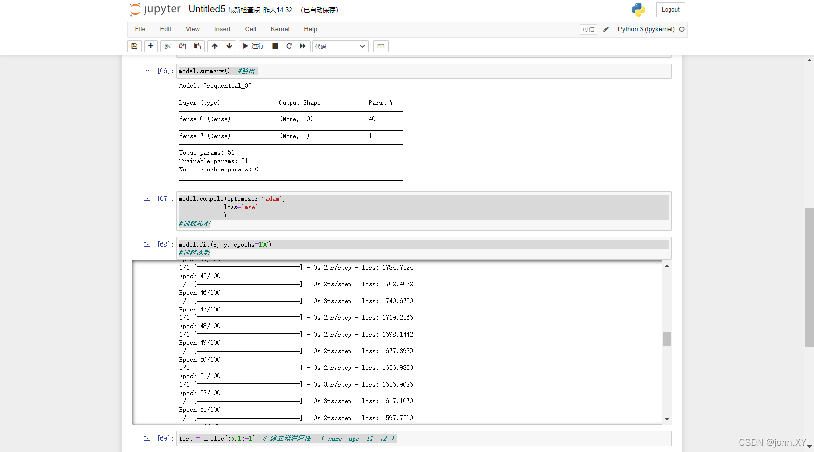
6
model.summary() #输出
7
model.compile(optimizer='adam',
             loss='mse'
             )
#训练模型
8
model.fit(x, y, epochs=100)
#训练次数
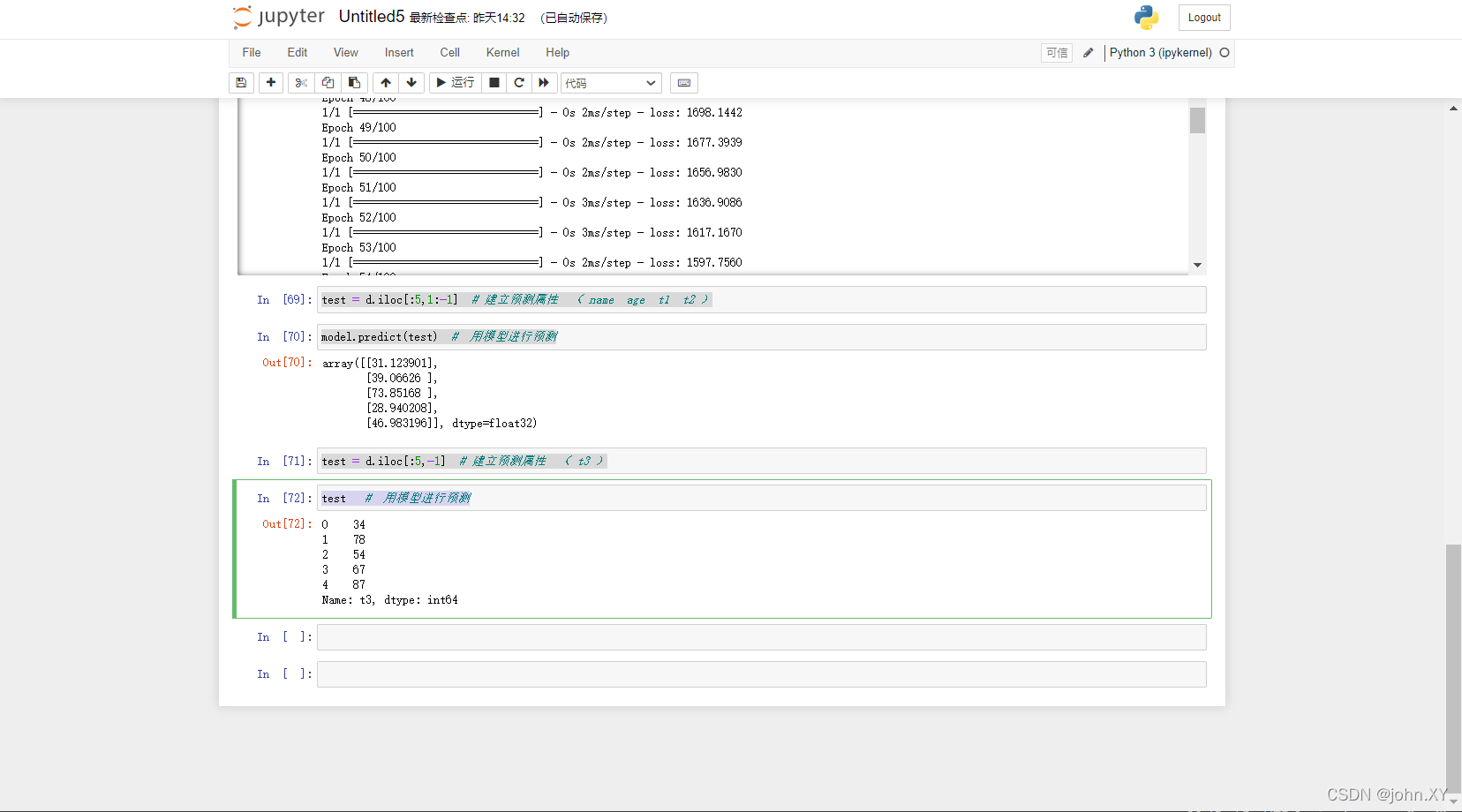
9
test = d.iloc[:5,1:-1] # 建立预测属性 ( name age t1 t2 )
10
model.predict(test) # 用模型进行预测
11
test = d.iloc[:5,-1] # 建立预测属性 ( t3 )
12
test # 用模型进行预测

···················································································································································································
目录
···················································································································································································