最近在复现论文时发现作者使用了 sklearn.metrics 库中的 average_precision_score() 函数用来对分类模型进行评价。
看了很多博文都未明白其原理与作用,看了sklean官方文档也未明白,直至在google上找到这篇文章Evaluating Object Detection Models Using Mean Average Precision (mAP),才恍然大悟,现作简单翻译与记录。
文章目录
- 从预测分数到类别标签(From Prediction Score to Class Label)
- 精确度-召回度曲线(Precision-Recall Curve)
- 平均精度AP(Average Precision)
- 总结
- 验证函数是否与该算法对照
- 结语
首先先说明一下计算的过程:
- 使用模型生成预测分数。
- 通过使用阈值将预测分数转化为类别标签。
- 计算混淆矩阵。
- 计算对应的精确率和召回率。
- 创建精确率-召回率曲线。
- 计算平均精度。
接下来分为三个阶段讲解:
从预测分数到类别标签(From Prediction Score to Class Label)
在本节中,我们将快速回顾一下如何从预测分数中派生出类标签。
假设有两个类别,Positive 和 Negative,这里是 10 个样本的真实标签。
y_true = ["positive", "negative", "negative", "positive", "positive", "positive", "negative", "positive", "negative", "positive"]
当这些样本被输入模型时,它会返回以下预测分数。基于这些分数,我们如何对样本进行分类(即为每个样本分配一个类标签)?
pred_scores = [0.7, 0.3, 0.5, 0.6, 0.55, 0.9, 0.4, 0.2, 0.4, 0.3]
为了将预测分数转换为类别标签,使用了一个阈值。当分数等于或高于阈值时,样本被归为一类(通常为正类, 1)。否则,它被归类为其他类别(通常为负类,0)。
以下代码块将分数转换为阈值为 0.5 的类标签。
import numpy

pred_scores = [0.7, 0.3, 0.5, 0.6, 0.55, 0.9, 0.4, 0.2, 0.4, 0.3]
y_true = ["positive", "negative", "negative", "positive", "positive", "positive", "negative", "positive", "negative", "positive"]

threshold = 0.5
y_pred = ["positive" if score >= threshold else "negative" for score in pred_scores]
print(y_pred)
转化后的标签如下:
['positive', 'negative', 'positive', 'positive', 'positive', 'positive', 'negative', 'negative', 'negative', 'negative']
现在 y_true 和 y_pred 变量中都提供了真实标签和预测标签。
基于这些标签,可以计算出混淆矩阵、精确率和召回率。(可以看这篇博文,讲得很不错,不过混淆矩阵那个图有点小瑕疵)
r = numpy.flip(sklearn.metrics.confusion_matrix(y_true, y_pred))
print(r)

precision = sklearn.metrics.precision_score(y_true=y_true, y_pred=y_pred, pos_label="positive")
print(precision)

recall = sklearn.metrics.recall_score(y_true=y_true, y_pred=y_pred, pos_label="positive")
print(recall)
其结果为
# Confusion Matrix (From Left to Right & Top to Bottom: True Positive, False Negative, False Positive, True Negative)
[[4 2]
 [1 3]]

# Precision = 4/(4+1)
0.8

# Recall = 4/(4+2)
0.6666666666666666
在快速回顾了计算准确率和召回率之后,接下来我们将讨论创建准确率-召回率曲线。
精确度-召回度曲线(Precision-Recall Curve)
根据给出的精度precision和召回率recall的定义,请记住,精度越高,模型将样本分类为阳性时的置信度就越高。召回率越高,模型正确分类为 Positive 的正样本就越多。
当一个模型具有高召回率但低精度时,该模型正确分类了大部分正样本,但它有很多误报(即将许多负样本分类为正样本)。当一个模型具有高精确度但低召回率时,该模型将样本分类为 Positive 时是准确的,但它可能只分类了一些正样本。
注:本人理解,要想一个模型真正达到优秀的效果,精确率和召回率都应较高。
由于准确率和召回率的重要性,一条准确率-召回率曲线可以显示不同阈值的准确率和召回率值之间的权衡。该曲线有助于选择最佳阈值以最大化两个指标。
创建精确召回曲线需要一些输入:
1. 真实标签。
2. 样本的预测分数。
3. 将预测分数转换为类别标签的一些阈值。
下一个代码块创建 y_true 列表来保存真实标签,pred_scores 列表用于预测分数,最后是用于不同阈值的 thresholds 列表。
import numpy

y_true = ["positive", "negative", "negative", "positive", "positive", "positive", "negative", "positive", "negative", "positive", "positive", "positive", "positive", "negative", "negative", "negative"]

pred_scores = [0.7, 0.3, 0.5, 0.6, 0.55, 0.9, 0.4, 0.2, 0.4, 0.3, 0.7, 0.5, 0.8, 0.2, 0.3, 0.35]

thresholds = numpy.arange(start=0.2, stop=0.7, step=0.05)
这是保存在阈值列表中的阈值。因为有 10 个阈值,所以将创建 10 个精度和召回值。
[0.2,
 0.25,
 0.3,
 0.35,
 0.4,
 0.45,
 0.5,
 0.55,
 0.6,
 0.65]
下一个名为 precision_recall_curve() 的函数接收真实标签、预测分数和阈值。它返回两个代表精度和召回值的等长列表。
import sklearn.metrics

def precision_recall_curve(y_true, pred_scores, thresholds):
    precisions = []
    recalls = []

    for threshold in thresholds:
        y_pred = ["positive" if score >= threshold else "negative" for score in pred_scores]

        precision = sklearn.metrics.precision_score(y_true=y_true, y_pred=y_pred, pos_label="positive")
        recall = sklearn.metrics.recall_score(y_true=y_true, y_pred=y_pred, pos_label="positive")

        precisions.append(precision)
        recalls.append(recall)

    return precisions, recalls
以下代码在传递三个先前准备好的列表后调用 precision_recall_curve() 函数。它返回精度和召回列表,分别包含精度和召回的所有值。
precisions, recalls = precision_recall_curve(y_true=y_true,
                                             pred_scores=pred_scores,
                                             thresholds=thresholds)
以下是精度precision列表中的返回值
[0.5625,
 0.5714285714285714,
 0.5714285714285714,
 0.6363636363636364,
 0.7,
 0.875,
 0.875,
 1.0,
 1.0,
 1.0]
这是召回recall列表中的值列表
[1.0,
 0.8888888888888888,
 0.8888888888888888,
 0.7777777777777778,
 0.7777777777777778,
 0.7777777777777778,
 0.7777777777777778,
 0.6666666666666666,
 0.5555555555555556,
 0.4444444444444444]
给定两个长度相等的列表,可以在二维图中绘制它们的值,如下所示
matplotlib.pyplot.plot(recalls, precisions, linewidth=4, color="red")
matplotlib.pyplot.xlabel("Recall", fontsize=12, fontweight='bold')
matplotlib.pyplot.ylabel("Precision", fontsize=12, fontweight='bold')
matplotlib.pyplot.title("Precision-Recall Curve", fontsize=15, fontweight="bold")
matplotlib.pyplot.show()
准确率-召回率曲线如下图所示。请注意,随着召回率的增加,精度会降低。原因是当正样本数量增加(高召回率)时,正确分类每个样本的准确率降低(低精度)。这是预料之中的,因为当有很多样本时,模型更有可能失败。
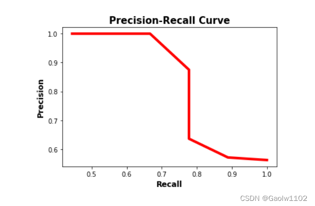
准确率-召回率曲线可以很容易地确定准确率和召回率都高的点。根据上图,最好的点是(recall, precision)=(0.778, 0.875)。
使用上图以图形方式确定精度和召回率的最佳值可能有效,因为曲线并不复杂。更好的方法是使用称为 f1 分数(f1-score) 的指标,它是根据下一个等式计算的。
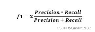
f1 指标衡量准确率和召回率之间的平衡。当 f1 的值很高时,这意味着精度和召回率都很高。较低的 f1 分数意味着精确度和召回率之间的失衡更大。
根据前面的例子,f1是根据下面的代码计算出来的。根据 f1 列表中的值,最高分是 0.82352941。它是列表中的第 6 个元素(即索引 5)。召回率和精度列表中的第 6 个元素分别为 0.778 和 0.875。对应的阈值为0.45。
f1 = 2 * ((numpy.array(precisions) * numpy.array(recalls)) / (numpy.array(precisions) + numpy.array(recalls)))
结果如下
[0.72,
 0.69565217,
 0.69565217,
 0.7,
 0.73684211,
 0.82352941,
 0.82352941,
 0.8,
 0.71428571,
 0.61538462]
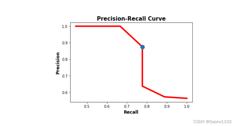
下图以蓝色显示了与召回率和准确率之间的最佳平衡相对应的点的位置。总之,平衡精度和召回率的最佳阈值是 0.45,此时精度为 0.875,召回率为 0.778。
matplotlib.pyplot.plot(recalls, precisions, linewidth=4, color="red", zorder=0)
matplotlib.pyplot.scatter(recalls[5], precisions[5], zorder=1, linewidth=6)

matplotlib.pyplot.xlabel("Recall", fontsize=12, fontweight='bold')
matplotlib.pyplot.ylabel("Precision", fontsize=12, fontweight='bold')
matplotlib.pyplot.title("Precision-Recall Curve", fontsize=15, fontweight="bold")
matplotlib.pyplot.show()
在讨论了精度-召回曲线之后,接下来讨论如何计算平均精度。
平均精度AP(Average Precision)
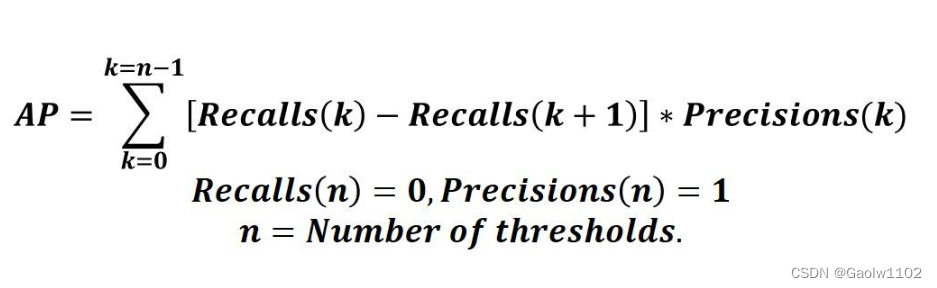
平均精度(AP)是一种将精度-召回曲线总结为代表所有精度平均值的单一数值的方法。 AP是根据下面的公式计算的。使用一个循环,通过遍历所有的精度precision/召回recall,计算出当前召回和下一次召回之间的差异,然后乘以当前精度。换句话说,Average-Precision是每个阈值的精确度(precision)的加权求和,其中的权重是召回率(recall)的差。
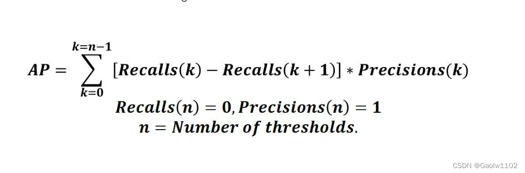
重要的是,要将召回列表recalls和精确列表precisions分别附加上0和1。例如,如果recalls列表是
0.8
,
0.6
0.8, 0.6
0.8,0.6
为它追加上 0, 就是
0.8
,
0.6
,
0.0
0.8, 0.6, 0.0
0.8,0.6,0.0
同样的,在精度列表precsion中附加1,
0.8
,
0.2
,
1.0
0.8, 0.2, 1.0
0.8,0.2,1.0
鉴于recalls和precisions都是NumPy数组,以上方程根据以下公式执行
AP = numpy.sum((recalls[:-1] - recalls[1:]) * precisions[:-1])
下面是计算AP的完整代码
import numpy
import sklearn.metrics

def precision_recall_curve(y_true, pred_scores, thresholds):
    precisions = []
    recalls = []

    for threshold in thresholds:
        y_pred = ["positive" if score >= threshold else "negative" for score in pred_scores]

        precision = sklearn.metrics.precision_score(y_true=y_true, y_pred=y_pred, pos_label="positive")
        recall = sklearn.metrics.recall_score(y_true=y_true, y_pred=y_pred, pos_label="positive")

        precisions.append(precision)
        recalls.append(recall**

    return precisions, recalls

y_true = ["positive", "negative", "negative", "positive", "positive", "positive", "negative", "positive", "negative", "positive", "positive", "positive", "positive", "negative", "negative", "negative"]
pred_scores = [0.7, 0.3, 0.5, 0.6, 0.55, 0.9, 0.4, 0.2, 0.4, 0.3, 0.7, 0.5, 0.8, 0.2, 0.3, 0.35]
thresholds=numpy.arange(start=0.2, stop=0.7, step=0.05)

precisions, recalls = precision_recall_curve(y_true=y_true,
                                             pred_scores=pred_scores,
                                             thresholds=thresholds)

precisions.append(1)
recalls.append(0)

precisions = numpy.array(precisions)
recalls = numpy.array(recalls)

AP = numpy.sum((recalls[:-1] - recalls[1:]) * precisions[:-1])
print(AP)
总结
需要注意的是,在 average_precision_score() 函数中,做了一些算法上的调整,与上不同,会将每一个预测分数作为阈值计算对应的精确率precision和召回率recall。最后在长度为 len(预测分数) 的precisions和recalls列表上,应用 Average-Precision 公式,得到最终 Average-Precision 值。
验证函数是否与该算法对照
现在从sklean的官方文档中,得到该函数的使用用例,如下(官方链接)
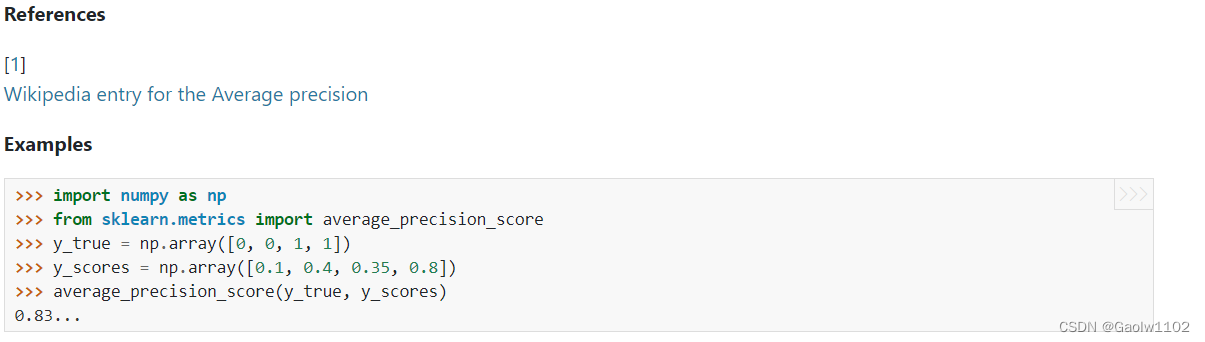
现在用以上的算法思想计算
import sklearn.metrics

'''
计算在给定阈值thresholds下的所有精确率与召回率
'''
def precision_recall_curve(y_true, pred_scores, thresholds):
    precisions = []
    recalls = []

    for threshold in thresholds:
        y_pred = [1 if score >= threshold else 0 for score in pred_scores]                           # 对此处稍微做修改
        print('y_true is:', y_true)
        print('y_pred is:', y_pred)

        confusion_matrix = sklearn.metrics.confusion_matrix(y_true, y_pred)                          # 输出混淆矩阵
        precision = sklearn.metrics.precision_score(y_true=y_true, y_pred=y_pred)                    # 输出精确率
        recall = sklearn.metrics.recall_score(y_true=y_true, y_pred=y_pred)                          # 输出召回率

        print('confusion_matrix is:', confusion_matrix)
        print('precision is:', precision)
        print('recall is:', recall)

        precisions.append(precision)
        recalls.append(recall)                                                                       # 追加精确率与召回率

        print('\n')

    return precisions, recalls
计算每个阈值对应的精确率与召回率,最后得到precisions, recalls
precisions, recalls = precision_recall_curve([0, 0, 1, 1], [0.1, 0.4, 0.35, 0.8], [0.1, 0.4, 0.35, 0.8])

'''
结果
y_true is: [0, 0, 1, 1]
y_pred is: [1, 1, 1, 1]
confusion_matrix is: [[0 2] [0 2]]
precision is: 0.5
recall is: 1.0


y_true is: [0, 0, 1, 1]
y_pred is: [0, 1, 0, 1]
confusion_matrix is: [[1 1] [1 1]]
precision is: 0.5
recall is: 0.5


y_true is: [0, 0, 1, 1]
y_pred is: [0, 1, 1, 1]
confusion_matrix is: [[1 1] [0 2]]
precision is: 0.6666666666666666
recall is: 1.0


y_true is: [0, 0, 1, 1]
y_pred is: [0, 0, 0, 1]
confusion_matrix is: [[2 0] [1 1]]
precision is: 1.0
recall is: 0.5
'''
precisions列表与recalls列表分别追加1, 0,输出precisions列表与recalls列表
precisions.append(1), recalls.append(0)
precisions, recalls
'''
结果
([0.5, 0.5, 0.6666666666666666, 1.0, 1], [1.0, 0.5, 1.0, 0.5, 0])
'''
代入Average-Precision公式,得
avg_precision = 0                                         # 初始化结果为0

# 不断加权求和
for i in range(len(precisions)-1):
    avg_precision += precisions[i] * (recalls[i] - recalls[i+1])

print('avg_precision is:', avg_precision)                 # 输出结果
输出结果为
avg_precision is: 0.8333333333333333
可以看到,和sklearn.matrics.average_precision_score()算法的执行结果一致,故正确。
结语
以上内容均为认真查看资料并计算得出的,可能会存在不正确的地方,如有小伙伴存在异议,请留言评论!