2022 APMCM亚太数学建模竞赛 C题 全球是否变暖 思路及代码实现(持续更新完毕)

更新信息
2022-11-24 10:00 更新问题1和问题2 思路
2022-11-24 23:20 更新问题一代码
2022-11-25 11:00 更新问题二代码
相关链接
【2022 APMCM亚太数学建模竞赛 C题 全球是否变暖 问题一python代码实现】
【2022 APMCM亚太数学建模竞赛 C题 全球是否变暖 问题二python代码实现】
【代码及建模方案下载】
方法一:私信我
方法二:https://gitee.com/liumengdemayun/BetterBench-Shop
2 思路及题目
2.1 题目
全球变暖与否? 加拿大49.6°C的高温为地球北纬50°以上地区创造了新的气温记录,一周内就有数百人死于高温;美国加利福尼亚州死亡谷54.4°C,是地球上有记录以来的最高温度;科威特53.5°C,阳光直射下甚至超过70°C,中东很多国家超过50°C。
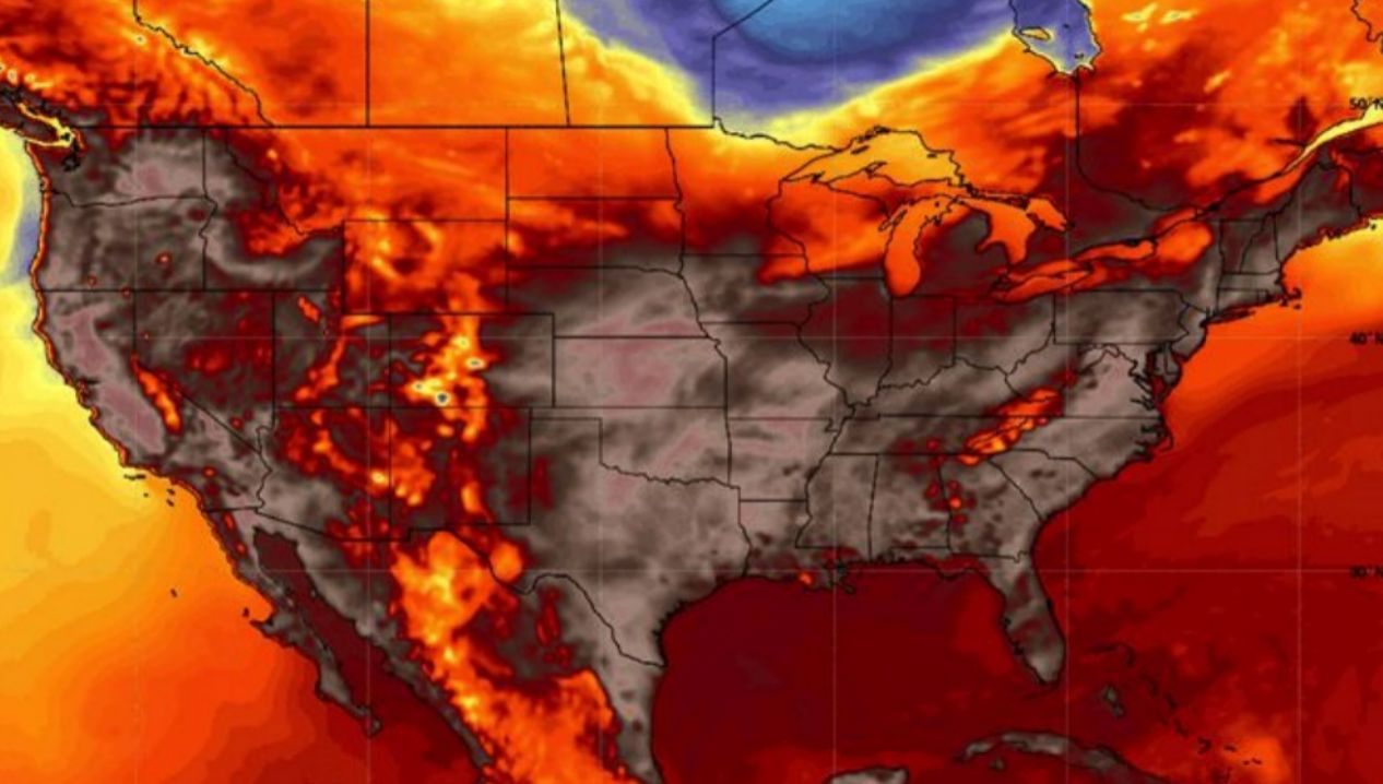
图1所示。北美的高温。 今年以来,我们看到了大量惊人的气温报告。地球正在燃烧的事实是毋庸置疑的。继这些地区从6月底到7月初的可怕高温之后,意大利再次创下欧洲气温纪录,达到惊人的48.8°C,许多国家宣布进入紧急状态。
全球气候变暖是一种与自然有关的现象。正是由于温室效应的不断积累,导致地球大气系统吸收和排放的能量失衡,能量在地球大气系统中不断积累,导致气温上升,全球气候变暖。
在工业革命之前,二氧化碳(CO2大气中的二氧化碳一直保持在280 ppm左右。2004年3月,大气中的二氧化碳浓度达到了377.7 ppm,这是到那时为止10年平均增幅最大的一次。根据美国国家海洋和大气管理局(NOAA)和斯克里普斯海洋学研究所(SIO)的科学家们的研究,月平均CO2 浓度水平在2022年5月达到峰值421 ppm。经济合作与发展组织(OECD)的一份报告预测CO2 到2050年,二氧化碳浓度将达到685 PPM
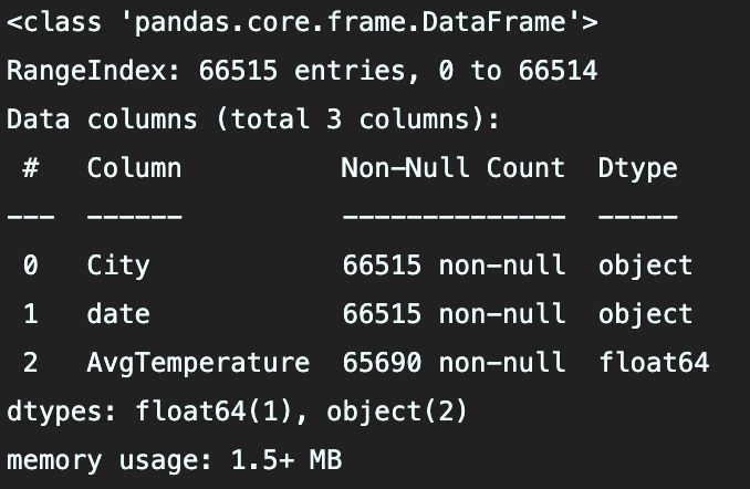
APMCM组委会已要求您的团队解决这些关于当前报告和未来全球温度水平预测的主张。他们提供了数据集2022_APMCM_C_Data.csv,其中包含239177条记录,以协助你们的研究。
需求 1.你同意全球温度的说法吗?使用附件中的2022_APMCM_C_Data.csv和你们团队收集的其他数据集来分析全球温度变化。
a)你是否同意2022年3月全球温度的上升导致了比以往任何10年期间观测到的更大的增长?为什么?为什么不? b)基于历史数据,请建立两个或两个以上的数学模型来描述过去并预测未来的全球温度水平。 c)分别使用1(b)中的每个模型来预测2050年和2100年的全球温度。你们的任何一个模型是否与2050年或2100年观测点的全球平均温度将达到20.00°C的预测一致?如果不是在2050年或2100年,你们预测模型中观测点的平均温度什么时候会达到20.00°C?
d)你在1(b)中建立的哪个模型你认为最准确?为什么? 2.影响温度变化的原因是什么? a)利用问题1的结果和附件2022_ APMCM_C_ data .csv和你们团队收集的其他数据集中的数据,建立一个数学模型来分析全球温度、时间和位置之间的关系(如果有),并解释它们之间的关系或证明它们之间没有关系。
b)请收集相关数据,分析自然灾害(如火山爆发、森林火灾和新冠肺炎)的因素。对全球气温有影响吗?
2.2 思路
(a)你是否同意2022年3月全球温度的上升导致了比以往任何10年期间观测到的更大的增长?为什么?为什么不?
思路:第一步,挑选几个城市,选取2022年的一整年的数据,将温度变化以折线图可视化,分析3月是不是存在异常值。
第二步,计算2022年排除3月的平均温度,和加上3月后的平均温度,计算2011年-2021年的平均温度,以折线图可视化。对比每年的增长,与2022年有无3月份数据的增长。
(b)基于历史数据,请建立两个或两个以上的数学模型来描述过去并预测未来的全球温度水平。
思路:从(c)知道,需要以年为跨度,建立时间序列预测模型。通过分析虽然有100个城市,但在题目中,没指定说明哪个观测点。
随机挑一个城市即可。以年为时间单位,统计每年的平均温度,得到一个时间序列。选择以下时间序列预测模型进行预测即可。注意题目需要两个模型。
有哪些时间序列预测模型
- 自回归 (AR)
- 移动平均线
- 自回归移动平均线
- 自回归积分移动平均线 (ARIMA)
- 季节性自回归积分移动平均线 (SARIMA)
- 具有外生回归量的季节性自回归综合移动平均线 (SARIMAX)
- 具有 ARIMA 误差的回归模型
- 向量自回归 (VAR)
- GARCH 模型
- Glostan、Jagannathan 和 Runkle GARCH 模型
(c)利用以上模型,预测未来100年的平均温度,并将这100个数据,可视化,分析什么时候能达到20度。
(d)模型的准确性,用评价指标来评价
模型的评价指标有
(1)MSE(mean squared error),是观测值(observed values)与预测值(predicted values)的误差的平方和的均值,即SSE/n。它是误差的二阶矩,包含估计量的方差(variance)及其偏差(bias),是衡量估计量质量的指标,其公式为:
(2)RMSE(root mean squared error),也称作RMSD(root mean square deviation),是MSE的算数平方根。由于每个误差(each error)对RMSD的影响与误差的平方(squared error)成正比,因此较大的误差会对RMSE影响过大,RMSE对异常值很敏感。其公式为:
(3)MAE(mean absolute error),是时间序列分析中预测误差常用的指标,由于MAE使用的是与被测数据相同的尺度(scale),因此不能用于比较两个不同尺度的序列。MAE又被称为L1范数损失函数(就是可以做为损失函数),是真实数据与预测数据之差的绝对值的均值。
(4)MAPE(mean absolute percentage error),也被称为MAPD(mean absolute percentage deviation),是一种衡量预测方法的预测准确性的指标。MAPE在解释相对误差(relative error)方面非常直观,在评价模型时MAPE通常用作回归(regression)问题的损失函数(loss function)。
3 代码实现
思路及Code下载:
GitHub - BetterBench
https://gitee.com/liumengdemayun/BetterBench-Shop
3.1 读取文件
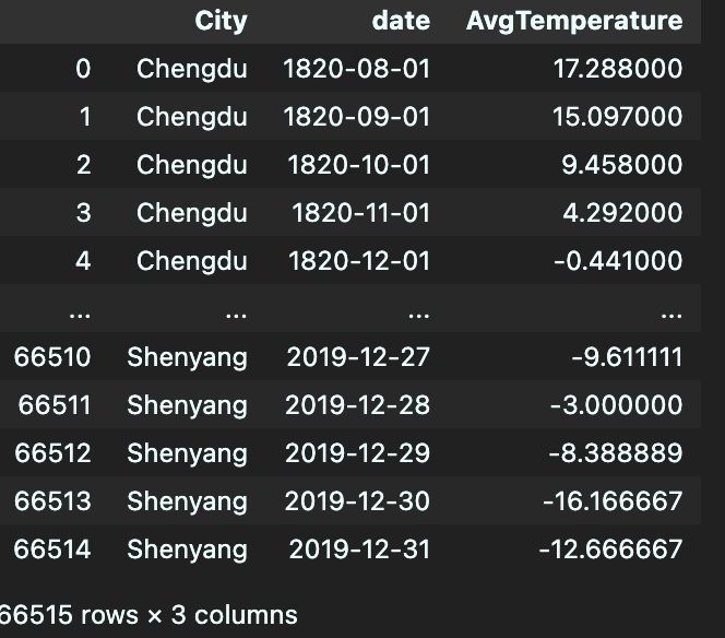
题目给的数据,只有到2013年的,我在网上找到了2013-2019的数据,合并上题目给的数据,从中选择中国部分城市,得到clear_China_city_AvgTemperature.csv,用于第一问分析,足够了
数据从1820至2019,剩下的2020-2022,采用手工查询
import pandas as pd
data = pd.read_csv('clear_China_city_AvgTemperature.csv')
data.head(10)
3.2 每年平均气温可视化
import matplotlib.pyplot as plt
import seaborn as sns

plt.figure(figsize = (22,25))
plt.subplot(4,1,1)
plt.plot(Chengdu_data.index, Chengdu_data['AvgTemperature'], 'g' ,label = 'Changchun')
plt.grid(linestyle = '--')
plt.legend(loc = 'best')
plt.title('Changchun Average Temperature')
plt.xlabel('Year')
plt.ylabel('AvgTemperature')

plt.subplot(4,1,2)
plt.plot(Shanghai_data.index, Shanghai_data['AvgTemperature'], 'r' ,label = 'Shanghai')
plt.grid(linestyle = '--')
plt.legend(loc = 'best')
plt.title('Shanghai Average Temperature')
plt.xlabel('Year')
plt.ylabel('AvgTemperature')
所有城市平均气温可视化
region = data[['City', 'Year', 'AvgTemperature']].groupby(['City','Year']).mean()

plt.figure(figsize = (14, 7))
plt.title('Average temperatures of City over the years 1994 to 2020')
sns.lineplot(x = 'Year', y = 'AvgTemperature', hue = 'City', units = 'City', markers = True, dashes = False, estimator = None, lw = 1, data = region)
plt.legend(bbox_to_anchor = (1, 1), shadow = True, fontsize = 'large', title = 'City')
plt.show()
3.3 10年滑动均线,平均气温可视化
# # 通过 https://www.tianqi24.com/chengdu/history202203.html查看
# 计算3月份时的平均气温是23度,不计算3月份的平均气温是11度
temp_df1 = pd.DataFrame({"AvgTemperature" :[22,23,22]},index=[2020,2021,2022])
temp_df2 = pd.DataFrame({"AvgTemperature" :[22,23,11]},index=[2020,2021,2022])
Chengdu_data_have3 = Chengdu_data.append(temp_df1)
Chengdu_data_nothave3 = Chengdu_data.append(temp_df2)


Chengdu_data_have3['Moving Average'] = Chengdu_data_have3['AvgTemperature'].rolling(10).mean()
Chengdu_data_nothave3['Moving Average'] = Chengdu_data_nothave3['AvgTemperature'].rolling(10).mean()
city_data1 = Chengdu_data_have3[-100:]
city_data2 = Chengdu_data_nothave3[-100:]
fig, ax = plt.subplots(figsize = (14, 7))
x = city_data1.index
y1 = city_data1['Moving Average']
ax.plot(x, y1, label='Moving-Average have 3Month')
y2 = city_data2['Moving Average']
ax.plot(x, y2, label='Moving-Average have not 3Month')
ax.legend()
从图中可以看到10年的滑动平均,在考虑了3月的气温突增后,观测值有明显的增大
3.4 建立预测模型
(1)数据可视化分析
import pandas as pd

data = pd.read_csv('2022_APMCM_C_Data.csv',encoding= 'unicode_escape')
data['dt'] = pd.to_datetime(data['dt'])
data['Year'] = data['dt'].dt.year
region = data[['City', 'Year', 'AverageTemperature']].groupby(['City','Year']).mean()

plt.figure(figsize = (14, 7))
plt.title('Average temperatures of City over the years 1743 to 2013')
sns.lineplot(x = 'Year', y = 'AverageTemperature', hue = 'City', units = 'City', markers = True, dashes = False, estimator = None, lw = 1, data = region)
plt.legend(bbox_to_anchor = (1, 1), shadow = True, fontsize = 'large', title = 'City')
plt.show()
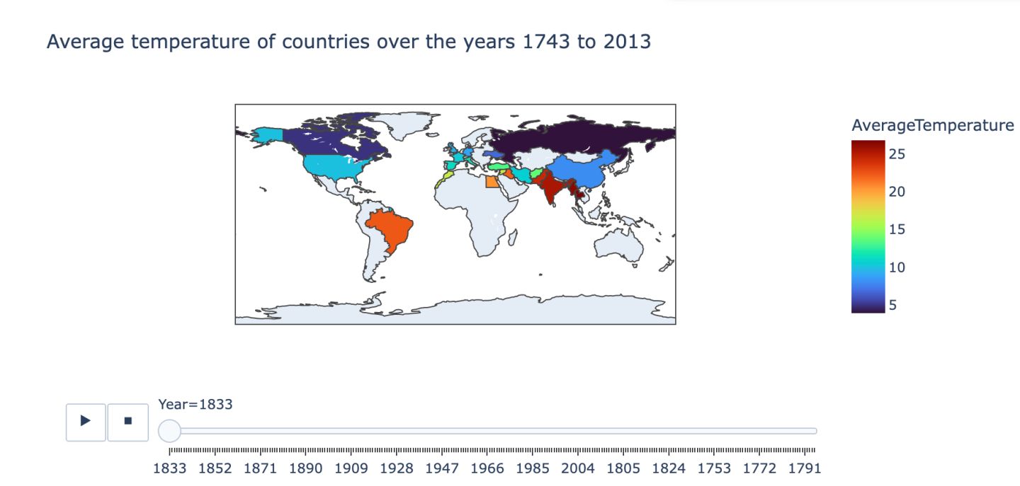
# pip install plotly==5.11.0
import plotly.express as px

temp_data = data[['Country','Year','AverageTemperature']].groupby(['Country','Year']).mean().reset_index()
px.choropleth(data_frame=temp_data,locations="Country",locationmode='country names',animation_frame="Year",color='AverageTemperature',color_continuous_scale = 'Turbo',title="Average temperature of countries over the years 1743 to 2013")
(2)以中国的数据进行建模
import matplotlib.pyplot as plt
import seaborn as sns
China_data = pd.read_csv('clear_China_city_AvgTemperature.csv')
China_data.head(10)
China_data.index =pd.to_datetime(China_data['date'])
Beijing_data = China_data[China_data['City'] == 'Beijing']
Guangzhou_data = China_data[China_data['City'] == 'Guangzhou']

# 异常值查看
for i in Beijing_data[['AvgTemperature']]:
    plt.figure()
    sns.boxplot(data[i])
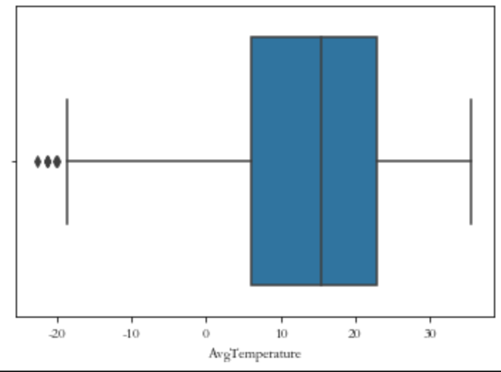
import numpy as np
Beijing_data['AvgTemperature'][Beijing_data['AvgTemperature']<-18]=np.nan
# 使用垂直方向的向前填充去填充空值
Beijing_data = Beijing_data.fillna(method = 'ffill',axis=0)
Guangzhou_data = Guangzhou_data.fillna(method = 'ffill',axis=0)
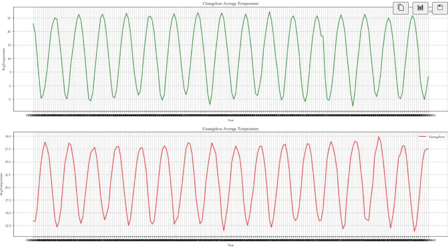
s = 0
e = 200
plt.figure(figsize = (22,25))
plt.subplot(4,1,1)
plt.plot(Beijing_data['date'][s:e], Beijing_data['AvgTemperature'][s:e], 'g' ,label = 'Changchun')
plt.grid(linestyle = '--')
plt.legend(loc = 'best')
plt.title('Changchun Average Temperature')
plt.xlabel('Year')
plt.ylabel('AvgTemperature')
plt.subplot(4,1,2)
plt.plot(Guangzhou_data['date'][s:e], Guangzhou_data['AvgTemperature'][s:e], 'r' ,label = 'Guangzhou')
plt.grid(linestyle = '--')
plt.legend(loc = 'best')
plt.title('Guangzhou Average Temperature')
plt.xlabel('Year')
plt.ylabel('AvgTemperature')
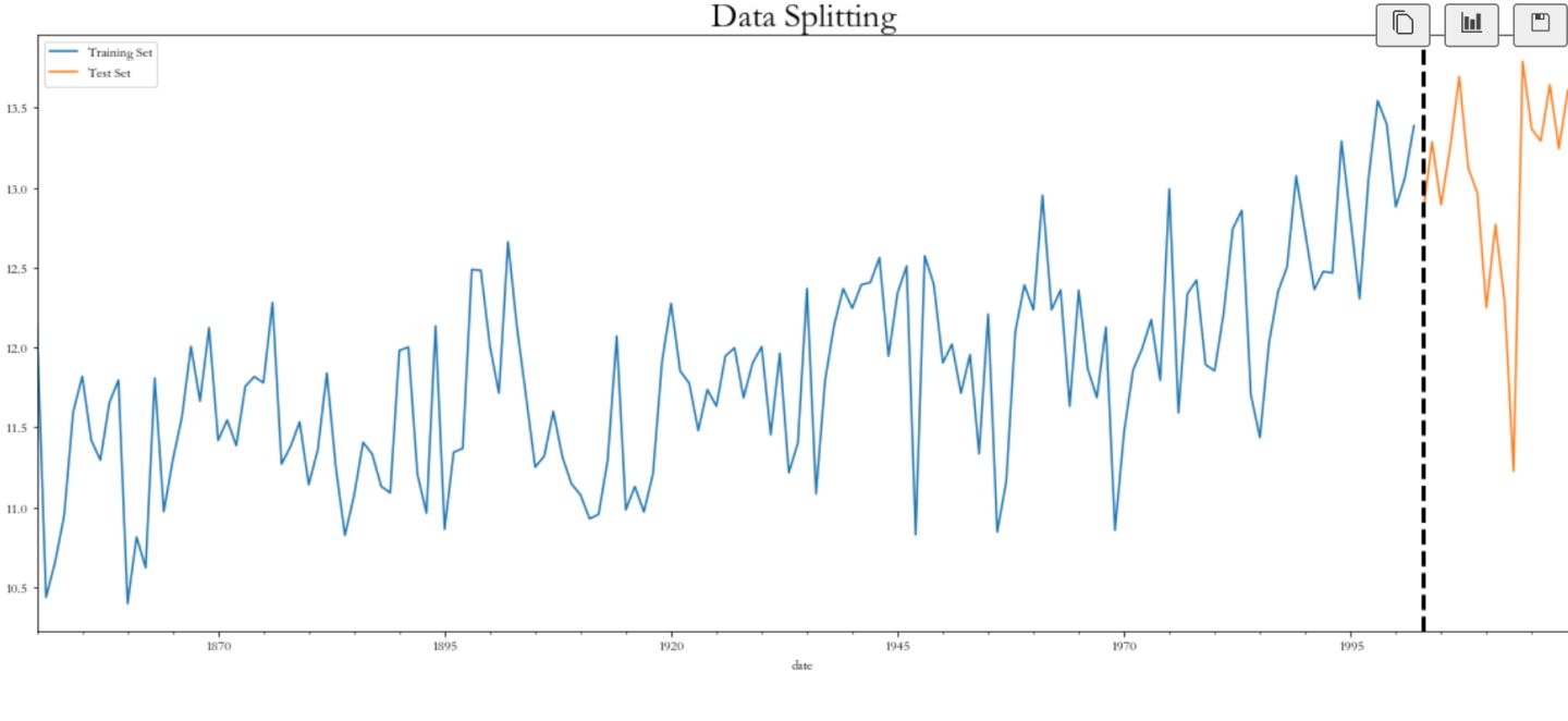
以年进行分组数据
Beijing_data.index = pd.to_datetime(Beijing_data['date'])
Beijing_data = Beijing_data[Beijing_data.index >'1850-01-01']
Beijing_data_df = Beijing_data.groupby(pd.Grouper(freq='Y')).mean()


df_train, df_test = Beijing_data_df[Beijing_data_df.index < '2003-01-01'], Beijing_data_df[Beijing_data_df.index >= '2003-01-01']
print('Train:\t', len(df_train))
print('Test:\t', len(df_test))
plt.figure(figsize=(20,8))

df_train['AvgTemperature'].plot(label='Training Set')
df_test['AvgTemperature'].plot(label='Test Set')
plt.axvline('2003-01-01', color='black', ls='--', lw=3)
plt.text('2003-02-01', 2, 'Split', fontsize=20, fontweight='bold')
plt.title('Data Splitting', weight='bold', fontsize=25)
plt.legend()
(3)模型一:Prophet预测
# pip install pystan==2.19.1.1
# pip install prophet -i https://pypi.douban.com/simple/
from prophet import Prophet
def index_to_column(data):
data['Datetime'] = data.index
data = data.sort_values('Datetime')
data = data.rename(columns={'Datetime': 'ds', 'AvgTemperature': 'y'})
return data
prophet_train = index_to_column(df_train)
prophet_test = index_to_column(df_test)
prophet_model = Prophet(interval_width=0.95)
prophet_model.fit(prophet_train)
prophet_pred = prophet_model.predict(prophet_test[['ds']]) # Keep the dataset format
from sklearn.metrics import mean_absolute_error
mae = round(mean_absolute_error(prophet_test['y'], prophet_pred['yhat']), 3)
print(mae)
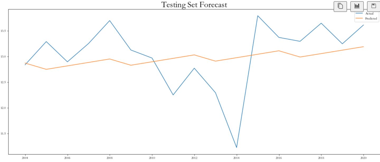
plt.figure(figsize=(20,8))
plt.plot(prophet_test['ds'], prophet_test['y'], label='Actual')
plt.plot(prophet_pred['ds'], prophet_pred['yhat'], label='Predicted')
plt.title('Test Forecasting', weight='bold', fontsize=40)
plt.title('Testing Set Forecast', weight='bold', fontsize=25)
plt.legend()
# 预测100后的温度
prophet_model2 = Prophet(interval_width=0.95)
prophet_model2.fit(prophet_train)
# 预测100年
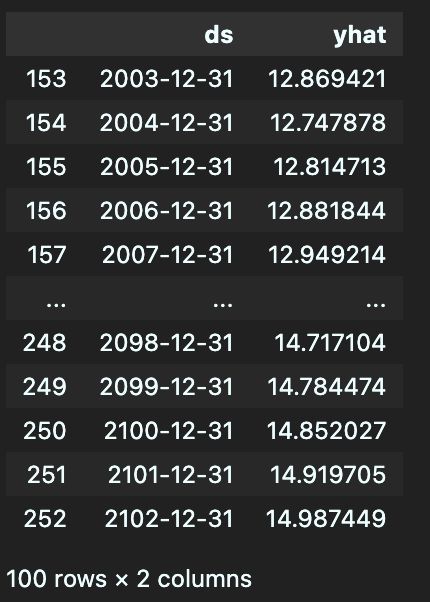
future_dates = prophet_model2.make_future_dataframe(periods=100, freq='Y')
prophet_pred2 = prophet_model2.predict(future_dates)
prophet_pred2[['ds','yhat']][-100:]
可以看到模型的mae为0.7,是比较大的了,模型准确性有待提高
(4)模型二:XGB预测
def date_transform(data):
df = data.copy()
df['Dayofweek'] = df.index.dayofweek
df['Dayofmonth'] = df.index.day
df['Dayofyear'] = df.index.dayofyear
df['weekofyear'] = df.index.weekofyear
df['Month'] = df.index.month
df['Quarter'] = df.index.quarter
df['Year'] = df.index.year
X = df.drop('AvgTemperature', axis=1)
y = df['AvgTemperature']
return X, y
Shenyang_data_df
df_train, df_test = Shenyang_data_df[Shenyang_data_df.index < '2003-01-01'], Shenyang_data_df[Shenyang_data_df.index >= '2003-01-01']
X_train, y_train = date_transform(df_train)
X_test, y_test = date_transform(df_test)
import xgboost as xgb
xgb_model = xgb.XGBRegressor(n_estimators=1000, learning_rate=0.05, early_stopping_rounds=10)
xgb_model.fit(X_train, y_train, eval_metric='mae', eval_set=[(X_train, y_train), (X_test, y_test)])
xgb_pred = xgb_model.predict(X_test)
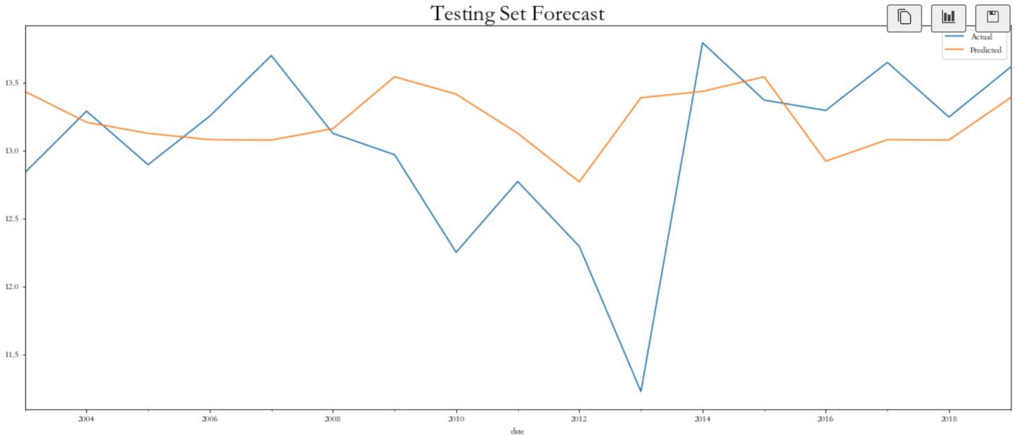
df_plot = pd.DataFrame({'y_test':y_test, 'xgb_pred':xgb_pred})
plt.figure(figsize=(20,8))
df_plot['y_test'].plot(label='Actual')
df_plot['xgb_pred'].plot(label='Predicted')
plt.title('Testing Set Forecast', weight='bold', fontsize=25)
plt.legend()
plt.show()
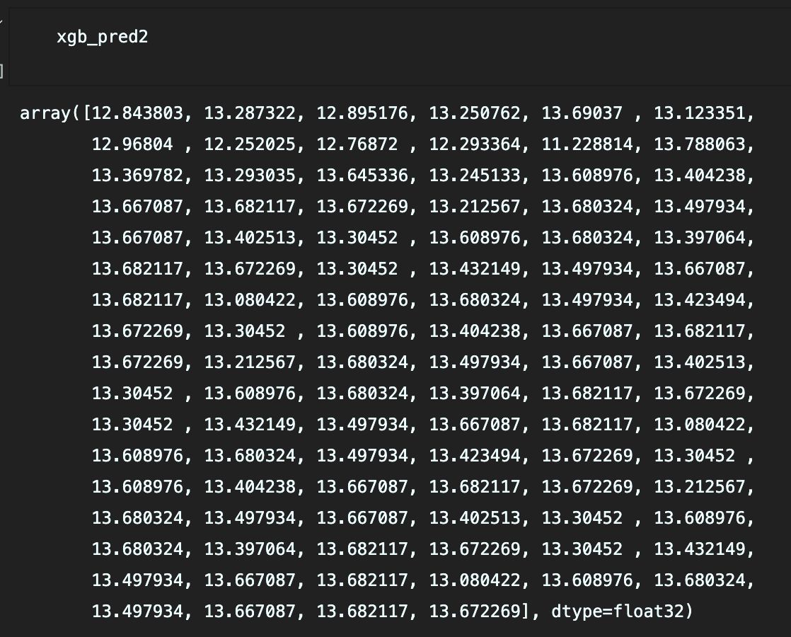
# 预测未来100年

import xgboost as xgb
future_dates2 = future_dates.iloc[-100:, :].copy()

future_dates2['ds'] = pd.to_datetime(future_dates2['ds'])
future_dates2 = future_dates2.set_index('ds')

future_dates2['Dayofweek'] = future_dates2.index.dayofweek
future_dates2['Dayofmonth'] = future_dates2.index.day
future_dates2['Dayofyear'] = future_dates2.index.dayofyear
future_dates2['weekofyear'] = future_dates2.index.weekofyear
future_dates2['Month'] = future_dates2.index.month
future_dates2['Quarter'] = future_dates2.index.quarter
future_dates2['Year'] = future_dates2.index.year

X_train, y_train = date_transform(df_train)
X_test, y_test = date_transform(df_test)
X = pd.concat([X_train, X_test], ignore_index=True)
y = pd.concat([y_train, y_test], ignore_index=True)

xgb_model2 = xgb.XGBRegressor(n_estimators=1000, learning_rate=0.05)
xgb_model2.fit(X, y, eval_metric='mae')
xgb_pred2 = xgb_model2.predict(future_dates2)


![[附源码]java毕业设计医院挂号管理系统](https://img-blog.csdnimg.cn/8c21c543cd494dc99b6e5d90f07cb824.png)