import torch
# PyTorch中初始化矩阵常见有以下几种方法
# 1. 直接使用固定值初始化
# M = torch.tensor([[1.0, 2.0, 3.0]]) # 1x3矩阵
# 2. 随机初始化
# M = torch.rand(1, 3) # 1x3矩阵,元素在0-1之间均匀分布
# M = torch.randn(1, 3) # 1x3矩阵,元素符合标准正态分布
# 3. 全零或全一初始化
# M = torch.zeros(1, 3) # 1x3全零矩阵
# M = torch.ones(1, 3) # 1x3全一矩阵
# 4. 从其他矩阵复制
# N = torch.ones_like(M) # 复制M的形状,元素全为1
# 初始化一个1 * 3 的矩阵M
M = torch.tensor([[1.0, 2.0, 3.0]])
# 初始化一个2 * 1 的矩阵N
N = torch.ones(2, 1)
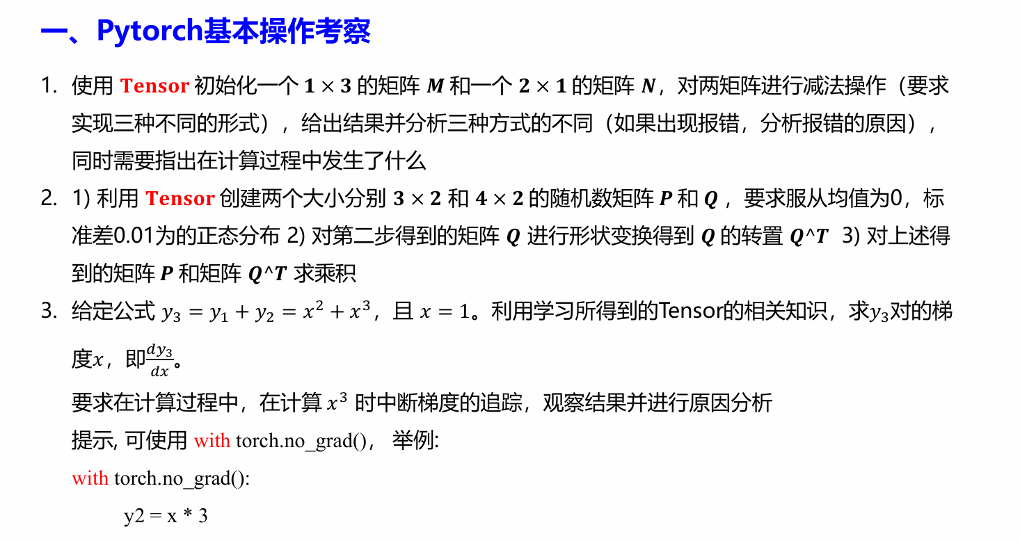
# 减法形式一
result1 = M - N
print(result1)
# 减法形式二
result2 = torch.sub(M, N)
print(result2)
# 减法形式三
a = torch.tensor([[1.0, 2.0, 3.0]])
b = torch.tensor([[1.0, 1.0, 1.0]])
a.sub_(b) # 直接在M上进行操作,修改M的值, 注意这里是in-place操作,会改变M的值
print(a) # 即M减去N后的结果,但M和N的形状必须相同
在PyTorch中,形状不同的矩阵相减是通过广播机制(Broadcasting)实现的,广播过程如下:
1. 比较维度:从右向左对齐
- M: (1,3)
- N: (2,1)
2. 扩展维度:
- 第0维:M的1扩展为2
- 第1维:N的1扩展为3
3. 最终计算时的形状:
- M扩展为 [[1,2,3], [1,2,3]] ,变为(2,3)
- N扩展为 [[1,1,1], [1,1,1]] ,变为(2,3)
4. 逐元素相减得到:
[[0,1,2], [0,1,2]]
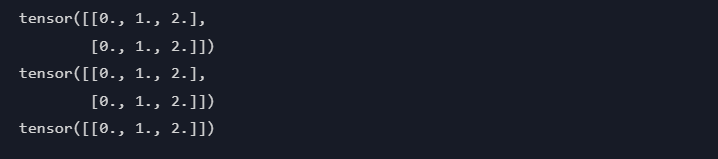
# 创建3×2的随机矩阵P,服从N(0,0.01)分布
P = torch.randn(3, 2) * 0.01
print("矩阵P:")
print(P)

# 创建4×2的随机矩阵Q,服从N(0,0.01)分布
Q = torch.randn(4, 2) * 0.01
print("矩阵Q:")
print(Q)

# 获取Q的转置(变为2×4)
Q_transpose = Q.T
print("Q的转置:")
print(Q_transpose)

# 计算P和Q转置的矩阵乘积(3×4)
result = torch.mm(P, Q_transpose)
print("P和Q转置的乘积:")
print(result)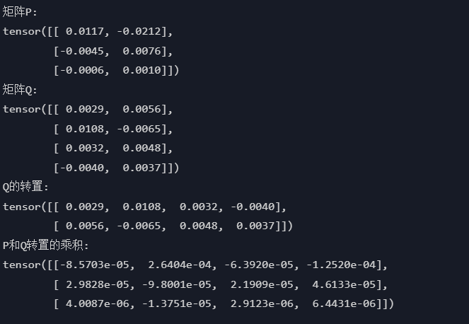
# 创建浮点型张量x
x = torch.tensor(1.0, requires_grad=True)
# 计算y1
y1 = x ** 2
# 计算y2时中断梯度
with torch.no_grad():
    y2 = x ** 3
# 计算y3
y3 = y1 + y2
# 计算梯度
y3.backward()
# 输出梯度
print(x.grad)  # 输出:tensor(2.)
注意:logistic回归虽然叫做回归,但实际被当作分类问题,通过取均值确定阈值,将标签转换成二分类(0或1)
手动实现logistic
import torch
from IPython import display
from matplotlib import pyplot as plt
import numpy as np
import random
# 设置随机种子,保证结果可复现
torch.manual_seed(42)
np.random.seed(42)
# 生成数据
num_inputs = 2
num_examples = 1000
true_w = [2, -3.4]
true_b = 4.2
features = torch.tensor(np.random.normal(0, 1, (num_examples, num_inputs)), dtype=torch.float)
labels = true_w[0] * features[:, 0] + true_w[1] * features[:, 1] + true_b
labels += torch.tensor(np.random.normal(0, 0.01, size=labels.size()), dtype=torch.float)
# 将连续标签转换为二分类标签
threshold = torch.mean(labels)
binary_labels = (labels > threshold).float().reshape(-1, 1)
# 划分训练集和测试集
train_size = int(0.8 * num_examples)
x_train, x_test = features[:train_size], features[train_size:]
y_train, y_test = binary_labels[:train_size], binary_labels[train_size:]
# 数据迭代器
def data_iter(batch_size, features, labels):
num_examples = len(features) # 样本总数
indices = list(range(num_examples)) # 生成样本索引列表
random.shuffle(indices) # 打乱样本顺序
for i in range(0, num_examples, batch_size): # 按批次生成样本索引
j = torch.LongTensor(indices[i: min(i + batch_size, num_examples)])
yield features.index_select(0, j), labels.index_select(0, j)
# 定义模型组件
def sigmoid(x):
return 1 / (1 + torch.exp(-x))
def logistic_regression(X, w, b):
return sigmoid(torch.mm(X, w) + b)
# 定义损失函数(二元交叉熵)
def binary_cross_entropy(y_hat, y):
return - (y * torch.log(y_hat + 1e-7) + (1 - y) * torch.log(1 - y_hat + 1e-7)).mean()
# 定义优化算法
def sgd(params, lr, batch_size):
for param in params:
param.data -= lr * param.grad / batch_size
# 初始化模型参数
w = torch.tensor(np.random.normal(0, 0.01, (num_inputs, 1)), dtype=torch.float, requires_grad=True)
b = torch.zeros(1, dtype=torch.float, requires_grad=True)
# 训练参数设置
lr = 0.03
num_epochs = 10
batch_size = 10
net = logistic_regression
loss = binary_cross_entropy
# 记录训练过程
train_losses = []
test_losses = []
train_accuracies = []
test_accuracies = []
# 模型训练
for epoch in range(num_epochs): # 遍历每个epoch
for X, y in data_iter(batch_size, x_train, y_train): # 遍历每个小批量
l = loss(net(X, w, b), y) # 计算损失
l.backward() # 反向传播计算梯度
sgd([w, b], lr, batch_size) # 更新参数
w.grad.data.zero_() # 梯度清零
b.grad.data.zero_() # 梯度清零
# 每个epoch评估一次模型
with torch.no_grad():
train_output = net(x_train, w, b) # 计算训练集上的输出
train_l = loss(train_output, y_train) # 计算训练集上的损失
train_pred = (train_output > 0.5).float() # 转换为二分类标签
train_accuracy = (train_pred == y_train).float().mean() # 计算训练集上的准确率
test_output = net(x_test, w, b) # 计算测试集上的输出
test_l = loss(test_output, y_test) # 计算测试集上的损失
test_pred = (test_output > 0.5).float() # 转换为二分类标签
test_accuracy = (test_pred == y_test).float().mean() # 计算测试集上的准确率
train_losses.append(train_l.item())
test_losses.append(test_l.item())
train_accuracies.append(train_accuracy.item())
test_accuracies.append(test_accuracy.item())
print(f'Epoch {epoch+1}, Train Loss: {train_l.item():.4f}, Test Loss: {test_l.item():.4f}')
print(f'Train Accuracy: {train_accuracy.item():.4f}, Test Accuracy: {test_accuracy.item():.4f}')
# 可视化训练过程
plt.figure(figsize=(12, 4))
plt.subplot(1, 2, 1)
plt.plot(train_losses, label='Train Loss')
plt.plot(test_losses, label='Test Loss')
plt.xlabel('Epoch')
plt.ylabel('Loss')
plt.legend()
plt.title('Training and Test Loss')
plt.subplot(1, 2, 2)
plt.plot(train_accuracies, label='Train Accuracy')
plt.plot(test_accuracies, label='Test Accuracy')
plt.xlabel('Epoch')
plt.ylabel('Accuracy')
plt.legend()
plt.title('Training and Test Accuracy')
plt.tight_layout()
plt.show()
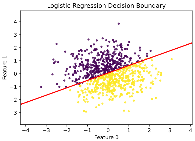
# 可视化决策边界
plt.figure(figsize=(6, 4))
plt.scatter(x_train[:, 0].numpy(), x_train[:, 1].numpy(), c=y_train.numpy().flatten(), cmap='viridis', s=10, alpha=0.8)
# 绘制决策边界
x_min, x_max = x_train[:, 0].min() - 1, x_train[:, 0].max() + 1
y_min, y_max = x_train[:, 1].min() - 1, x_train[:, 1].max() + 1
xx, yy = np.meshgrid(np.arange(x_min, x_max, 0.02), np.arange(y_min, y_max, 0.02))
grid_points = torch.tensor(np.c_[xx.ravel(), yy.ravel()], dtype=torch.float)
with torch.no_grad():
Z = net(grid_points, w, b).numpy()
Z = Z.reshape(xx.shape)
plt.contour(xx, yy, Z, levels=[0.5], linewidths=2, colors='r')
plt.title('Logistic Regression Decision Boundary')
plt.xlabel('Feature 0')
plt.ylabel('Feature 1')
plt.show()
# 输出最终参数
print(f'\n最终训练得到的参数:')
print(f'w: {w.detach().numpy().flatten()}')
print(f'b: {b.item()}')
print(f'真实参数:')
print(f'w: {true_w}')
print(f'b: {true_b}')

训练参数与真实参数差距分析
训练得到的参数w: [ 0.36611313 -0.64247864] 、b: 0.03421853110194206 与真实参数w: [2, -3.4] 、b: 4.2相比,差距是比较大的 。以下是造成差距的可能原因:
-
模型复杂度:Logistic 回归本质上是一个相对简单的线性分类模型。在此次任务中,虽然数据是基于线性关系构造,但 Logistic 回归的目标是分类(将连续标签转换为二分类 ),其拟合的是分类边界,和原始用于生成数据的线性回归关系存在本质区别。简单的模型结构可能不足以准确还原用于生成数据的真实参数关系。
-
数据噪声:生成数据时添加了服从均值为 0、标准差为 0.01 的正态分布噪声。噪声的存在使得数据偏离了原本纯粹由真实参数确定的关系,模型在训练过程中会学习到噪声的一些特征,干扰了对真实参数的逼近,导致训练参数和真实参数出现偏差。
-
训练轮数不足:此次训练设置的轮数为 10 轮,可能相对较少。模型还未充分收敛,没有足够的迭代次数去不断调整参数以接近真实参数。增加训练轮数,可能会使参数进一步优化,缩小与真实参数的差距。
-
学习率设置:学习率为 0.03 ,如果该值设置得过大,模型在参数更新时可能会 “跳过” 最优参数值,导致无法准确收敛到真实参数附近;若设置过小,参数更新步伐缓慢,在有限的训练轮数内也难以逼近真实参数 。
-
样本数量:尽管有 1000 个样本,但对于复杂的真实参数关系和存在噪声的数据,样本数量可能不够充足。样本数量不足可能导致模型无法全面捕捉数据背后真实参数所蕴含的规律,从而使训练参数偏离真实参数 。
利用torch.nn实现logistic
import torch
import torch.nn as nn
import torch.utils.data as Data
import numpy as np

# 生成人工构造数据集
num_inputs = 2
num_examples = 1000
true_w = [2, -3.4]
true_b = 4.2
features = torch.tensor(np.random.normal(0, 1, (num_examples, num_inputs)), dtype=torch.float)
labels = true_w[0] * features[:, 0] + true_w[1] * features[:, 1] + true_b
labels += torch.tensor(np.random.normal(0, 0.01, size=labels.size()), dtype=torch.float)
# 将连续标签转换为二分类标签
threshold = torch.mean(labels)
binary_labels = (labels > threshold).float().reshape(-1, 1)

# 划分训练集和测试集
train_size = int(0.8 * num_examples)
x_train, x_test = features[:train_size], features[train_size:]
y_train, y_test = binary_labels[:train_size], binary_labels[train_size:]

batch_size = 10
lr = 0.03
# 将训练数据的特征和标签组合
train_dataset = Data.TensorDataset(x_train, y_train)
# 把训练dataset放入DataLoader
train_data_iter = Data.DataLoader(
    dataset=train_dataset,
    batch_size=batch_size,
    shuffle=True,
    num_workers=0
)

# 定义模型
class LogisticNet(nn.Module):
    def __init__(self, n_feature):
        super(LogisticNet, self).__init__()
        self.linear = nn.Linear(n_feature, 1)
        self.sigmoid = nn.Sigmoid()  # 添加sigmoid激活函数

    def forward(self, x):
        x = self.linear(x)
        x = self.sigmoid(x)
        return x

net = LogisticNet(num_inputs)

# 模型参数初始化
from torch.nn import init
init.normal_(net.linear.weight, mean=0, std=0.01)
init.constant_(net.linear.bias, val=0)

# 定义损失函数
loss = nn.BCELoss()

# 定义优化算法
import torch.optim as optim
optimizer = optim.SGD(net.parameters(), lr=lr)

# 模型训练
num_epochs = 3
for epoch in range(num_epochs):
    for X, y in train_data_iter:
        output = net(X)
        l = loss(output, y)
        optimizer.zero_grad()
        l.backward()
        optimizer.step()
    print('epoch %d, loss: %f' % (epoch + 1, l.item()))

# 模型测试
with torch.no_grad():
    test_output = net(x_test)
    predicted = (test_output > 0.5).float()
    accuracy = (predicted == y_test).sum().item() / y_test.size(0)
    print(f"测试集准确率: {accuracy}")

    train_output = net(x_train)
    train_predicted = (train_output > 0.5).float()
    train_accuracy = (train_predicted == y_train).sum().item() / y_train.size(0)
    print(f"训练集准确率: {train_accuracy}")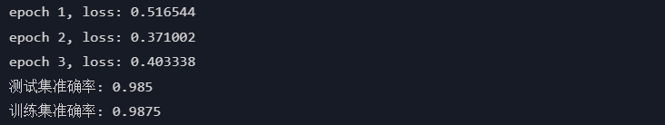

注意:Softmax 回归不是回归问题,而是多分类问题的分类算法。虽名字中有 “回归”,但本质与传统回归不同:
-
传统回归问题:像线性回归,旨在建立自变量和因变量间的定量关系,预测一个连续数值,例如根据房屋面积、房龄等预测房价,重点在数值预测 。
-
Softmax 回归:是 Logistic 回归在多分类场景的推广。对于输入数据,它通过 Softmax 函数将多个输出值转换为概率分布,每个概率代表样本属于对应类别的可能性,最终根据概率确定样本类别 。比如在手写数字识别中,将图像分类为 0 - 9 这 10 个数字类别之一。
Softmax 回归是通过计算样本属于各个类别的概率来实现分类,并非预测连续数值,所以不属于回归问题 。
手动实现softmax回归
import torch
import numpy as np
import matplotlib.pyplot as plt
from torchvision import datasets, transforms
# 数据预处理(添加更合理的标准化)
transform = transforms.Compose([
transforms.ToTensor(),
transforms.Normalize((0.1307,), (0.3081,)) # Fashion-MNIST的均值和标准差
])
# 加载训练集
train_dataset = datasets.FashionMNIST(root='./data', train=True,
download=True, transform=transform)
train_loader = torch.utils.data.DataLoader(train_dataset, batch_size=64,
shuffle=True)
# 加载测试集
test_dataset = datasets.FashionMNIST(root='./data', train=False,
download=True, transform=transform)
test_loader = torch.utils.data.DataLoader(test_dataset, batch_size=64,
shuffle=False)
# 数值稳定的Softmax函数
def softmax(X):
# 减去每行的最大值以防止指数运算溢出
X_max, _ = torch.max(X, dim=1, keepdim=True)
X = X - X_max
X_exp = torch.exp(X)
partition = X_exp.sum(dim=1, keepdim=True)
return X_exp / partition
# 数值稳定的交叉熵损失函数
def cross_entropy_loss(y_hat, y):
# 使用log_softmax更稳定
log_y_hat = torch.log(y_hat + 1e-10) # 添加小常数防止log(0)
num_examples = y_hat.shape[0]
loss = -log_y_hat[range(num_examples), y]
return loss.mean()
# 初始化模型参数(使用更合理的初始化)
num_inputs = 784
num_outputs = 10
# 使用Xavier初始化
W = torch.tensor(np.random.normal(0, np.sqrt(1/num_inputs), (num_inputs, num_outputs)),
dtype=torch.float, requires_grad=True)
b = torch.zeros(num_outputs, dtype=torch.float, requires_grad=True)
# 定义模型
def net(X):
X = X.view((-1, num_inputs))
return softmax(torch.matmul(X, W) + b)
# 定义优化算法(添加梯度裁剪防止梯度爆炸)
def sgd(params, lr, batch_size, grad_clip=1.0):
for param in params:
# 梯度裁剪
if param.grad is not None:
torch.nn.utils.clip_grad_norm_(param, grad_clip)
param.data -= lr * param.grad / batch_size
# 训练模型
lr = 0.1 # 调整学习率
num_epochs = 10 # 增加训练轮数
train_losses = []
train_accuracies = []
test_losses = []
test_accuracies = []
for epoch in range(num_epochs):
epoch_loss = 0.0
correct_count = 0
total_count = 0
for X, y in train_loader:
y_hat = net(X)
l = cross_entropy_loss(y_hat, y)
# 检查损失是否为nan
if torch.isnan(l):
print("检测到NaN损失,跳过此次更新")
continue
l.backward()
sgd([W, b], lr, X.shape[0])
# 梯度清零
for param in [W, b]:
if param.grad is not None:
param.grad.zero_()
with torch.no_grad():
epoch_loss += l.item() * X.shape[0]
predict_labels = y_hat.argmax(dim=1)
correct_count += (predict_labels == y).sum().item()
total_count += y.shape[0]
epoch_loss /= total_count
epoch_accuracy = correct_count / total_count
train_losses.append(epoch_loss)
train_accuracies.append(epoch_accuracy)
# 测试集评估
test_epoch_loss = 0.0
test_correct_count = 0
test_total_count = 0
for X, y in test_loader:
with torch.no_grad():
y_hat = net(X)
l = cross_entropy_loss(y_hat, y)
test_epoch_loss += l.item() * X.shape[0]
predict_labels = y_hat.argmax(dim=1)
test_correct_count += (predict_labels == y).sum().item()
test_total_count += y.shape[0]
test_epoch_loss /= test_total_count
test_epoch_accuracy = test_correct_count / test_total_count
test_losses.append(test_epoch_loss)
test_accuracies.append(test_epoch_accuracy)
print(f'Epoch {epoch + 1}: Train Loss: {epoch_loss:.4f}, Train Accuracy: {epoch_accuracy:.4f}, Test Loss: {test_epoch_loss:.4f}, Test Accuracy: {test_epoch_accuracy:.4f}')
# 绘制训练和测试损失曲线
plt.figure(figsize=(12, 5))
plt.subplot(1, 2, 1)
plt.plot(train_losses, label='Train Loss')
plt.plot(test_losses, label='Test Loss')
plt.xlabel('Epoch')
plt.ylabel('Loss')
plt.legend()
plt.title('Training and Test Loss')
# 绘制训练和测试准确率曲线
plt.subplot(1, 2, 2)
plt.plot(train_accuracies, label='Train Accuracy')
plt.plot(test_accuracies, label='Test Accuracy')
plt.xlabel('Epoch')
plt.ylabel('Accuracy')
plt.legend()
plt.title('Training and Test Accuracy')
plt.tight_layout()
plt.show()
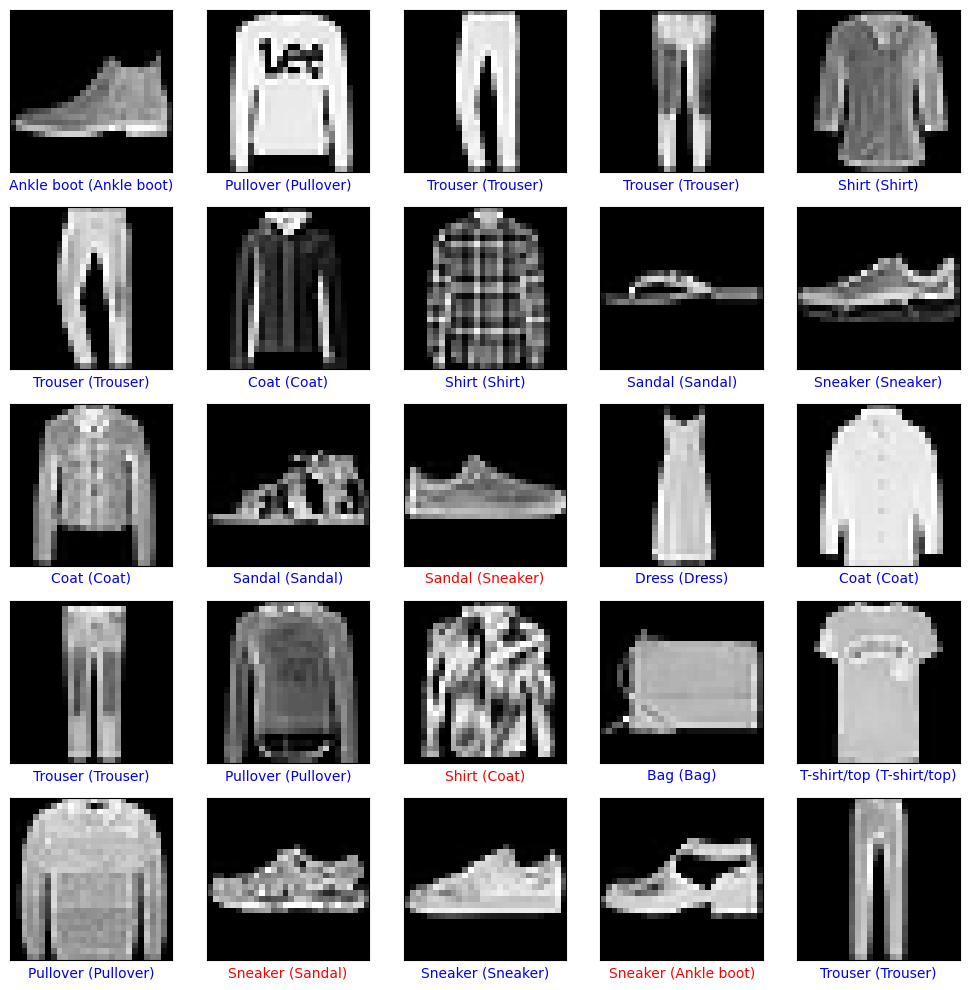
# 可视化预测结果
def visualize_predictions():
examples = iter(test_loader)
X, y = next(examples)
with torch.no_grad():
predictions = net(X).argmax(dim=1)
class_names = ['T-shirt/top', 'Trouser', 'Pullover', 'Dress', 'Coat',
'Sandal', 'Shirt', 'Sneaker', 'Bag', 'Ankle boot']
plt.figure(figsize=(10, 10))
for i in range(25):
plt.subplot(5, 5, i+1)
plt.xticks([])
plt.yticks([])
plt.grid(False)
plt.imshow(X[i][0].numpy(), cmap='gray')
if predictions[i] == y[i]:
color = 'blue'
else:
color = 'red'
plt.xlabel(f"{class_names[predictions[i]]} ({class_names[y[i]]})", color=color)
plt.tight_layout()
plt.show()
visualize_predictions()打印结果
Epoch 1: Train Loss: 1.4510, Train Accuracy: 0.5134, Test Loss: 0.9169, Test Accuracy: 0.7025
Epoch 2: Train Loss: 0.7942, Train Accuracy: 0.7412, Test Loss: 0.7369, Test Accuracy: 0.7537
Epoch 3: Train Loss: 0.6799, Train Accuracy: 0.7773, Test Loss: 0.6643, Test Accuracy: 0.7782
Epoch 4: Train Loss: 0.6249, Train Accuracy: 0.7922, Test Loss: 0.6239, Test Accuracy: 0.7890
Epoch 5: Train Loss: 0.5913, Train Accuracy: 0.8019, Test Loss: 0.5975, Test Accuracy: 0.7960
Epoch 6: Train Loss: 0.5680, Train Accuracy: 0.8090, Test Loss: 0.5790, Test Accuracy: 0.8024
Epoch 7: Train Loss: 0.5506, Train Accuracy: 0.8139, Test Loss: 0.5651, Test Accuracy: 0.8050
Epoch 8: Train Loss: 0.5371, Train Accuracy: 0.8179, Test Loss: 0.5542, Test Accuracy: 0.8093
Epoch 9: Train Loss: 0.5262, Train Accuracy: 0.8206, Test Loss: 0.5456, Test Accuracy: 0.8119
Epoch 10: Train Loss: 0.5171, Train Accuracy: 0.8235, Test Loss: 0.5375, Test Accuracy: 0.8131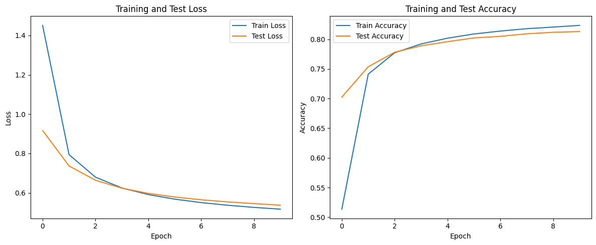
利用torch.nn实现softmax回归
import torch
import torch.nn as nn
import torch.optim as optim
import numpy as np
import matplotlib.pyplot as plt
from torchvision import datasets, transforms
# 设置随机种子,保证结果可复现
torch.manual_seed(42)
np.random.seed(42)
# 数据预处理
transform = transforms.Compose([
transforms.ToTensor(),
transforms.Normalize((0.1307,), (0.3081,)) # Fashion-MNIST的均值和标准差
])
# 加载训练集
train_dataset = datasets.FashionMNIST(root='./data', train=True,
download=True, transform=transform)
train_loader = torch.utils.data.DataLoader(train_dataset, batch_size=64,
shuffle=True)
# 加载测试集
test_dataset = datasets.FashionMNIST(root='./data', train=False,
download=True, transform=transform)
test_loader = torch.utils.data.DataLoader(test_dataset, batch_size=64,
shuffle=False)
# 定义Softmax回归模型
class SoftmaxRegression(nn.Module):
def __init__(self):
super(SoftmaxRegression, self).__init__()
self.fc = nn.Linear(784, 10)
self.dropout = nn.Dropout(0.2) # 添加Dropout层,丢弃概率设为0.2
def forward(self, x):
x = x.view(-1, 784)
x = self.dropout(x) # 在前向传播中使用Dropout
return self.fc(x)
# 初始化模型、损失函数和优化器
model = SoftmaxRegression()
criterion = nn.CrossEntropyLoss()
optimizer = optim.SGD(model.parameters(), lr=0.1)
# 训练模型
num_epochs = 10
train_losses = []
train_accuracies = []
test_losses = []
test_accuracies = []
for epoch in range(num_epochs):
model.train() # 设置为训练模式
running_loss = 0.0
correct = 0
total = 0
for batch_idx, (data, target) in enumerate(train_loader):
optimizer.zero_grad()
output = model(data)
loss = criterion(output, target)
loss.backward()
optimizer.step()
running_loss += loss.item()
_, predicted = output.max(1)
total += target.size(0)
correct += predicted.eq(target).sum().item()
epoch_loss = running_loss / (batch_idx + 1)
epoch_accuracy = correct / total
train_losses.append(epoch_loss)
train_accuracies.append(epoch_accuracy)
model.eval() # 设置为评估模式
test_running_loss = 0.0
test_correct = 0
test_total = 0
with torch.no_grad():
for data, target in test_loader:
output = model(data)
test_loss = criterion(output, target)
test_running_loss += test_loss.item()
_, test_predicted = output.max(1)
test_total += target.size(0)
test_correct += test_predicted.eq(target).sum().item()
test_epoch_loss = test_running_loss / len(test_loader)
test_epoch_accuracy = test_correct / test_total
test_losses.append(test_epoch_loss)
test_accuracies.append(test_epoch_accuracy)
print(f'Epoch {epoch + 1}: Train Loss: {epoch_loss:.4f}, Train Accuracy: {epoch_accuracy:.4f}, Test Loss: {test_epoch_loss:.4f}, Test Accuracy: {test_epoch_accuracy:.4f}')
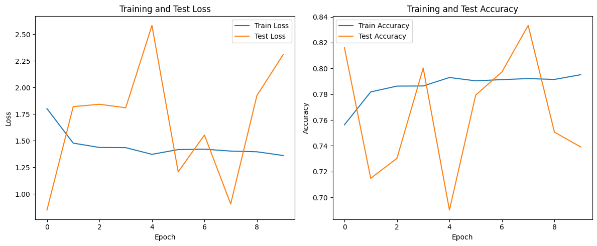
# 可视化训练结果
plt.figure(figsize=(12, 5))
plt.subplot(1, 2, 1)
plt.plot(train_losses, label='Train Loss')
plt.plot(test_losses, label='Test Loss')
plt.xlabel('Epoch')
plt.ylabel('Loss')
plt.legend()
plt.title('Training and Test Loss')
plt.subplot(1, 2, 2)
plt.plot(train_accuracies, label='Train Accuracy')
plt.plot(test_accuracies, label='Test Accuracy')
plt.xlabel('Epoch')
plt.ylabel('Accuracy')
plt.legend()
plt.title('Training and Test Accuracy')
plt.tight_layout()
plt.show()
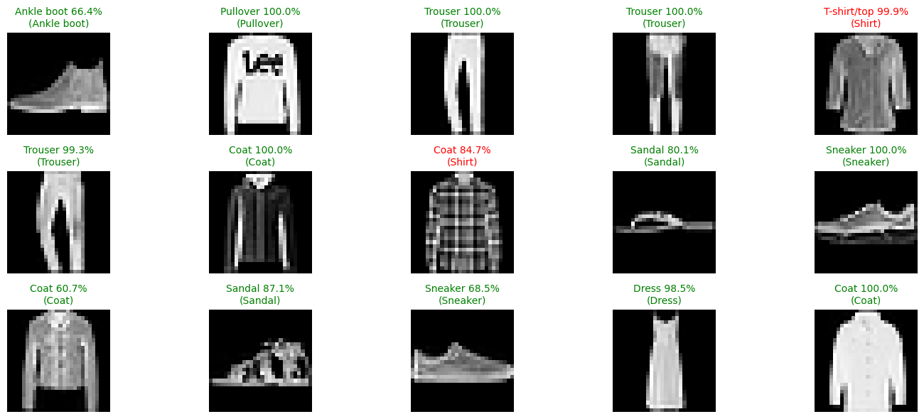
# 可视化预测结果
def visualize_predictions(model, test_loader, num_samples=15):
class_names = ['T-shirt/top', 'Trouser', 'Pullover', 'Dress', 'Coat',
'Sandal', 'Shirt', 'Sneaker', 'Bag', 'Ankle boot']
examples = iter(test_loader)
data, targets = next(examples)
model.eval()
with torch.no_grad():
outputs = model(data)
probs = torch.nn.functional.softmax(outputs, dim=1)
predictions = outputs.argmax(dim=1)
plt.figure(figsize=(15, 6))
for i in range(num_samples):
plt.subplot(3, 5, i+1)
# 显示图像
img = data[i].squeeze().numpy()
img = img * 0.3081 + 0.1307 # 反标准化
plt.imshow(img, cmap='gray')
plt.axis('off')
# 获取预测概率和真实标签
prob = probs[i][predictions[i]].item() * 100
pred_class = class_names[predictions[i]]
true_class = class_names[targets[i]]
# 设置标题颜色(正确为绿色,错误为红色)
color = 'green' if predictions[i] == targets[i] else 'red'
plt.title(f'{pred_class} {prob:.1f}%\n({true_class})', color=color, fontsize=10)
plt.tight_layout()
plt.show()
# 可视化预测结果
visualize_predictions(model, test_loader)Epoch 1: Train Loss: 1.8012, Train Accuracy: 0.7563, Test Loss: 0.8480, Test Accuracy: 0.8160
Epoch 2: Train Loss: 1.4771, Train Accuracy: 0.7818, Test Loss: 1.8200, Test Accuracy: 0.7148
Epoch 3: Train Loss: 1.4363, Train Accuracy: 0.7863, Test Loss: 1.8425, Test Accuracy: 0.7303
Epoch 4: Train Loss: 1.4345, Train Accuracy: 0.7864, Test Loss: 1.8095, Test Accuracy: 0.8003
Epoch 5: Train Loss: 1.3718, Train Accuracy: 0.7930, Test Loss: 2.5834, Test Accuracy: 0.6902
Epoch 6: Train Loss: 1.4163, Train Accuracy: 0.7904, Test Loss: 1.2069, Test Accuracy: 0.7793
Epoch 7: Train Loss: 1.4203, Train Accuracy: 0.7913, Test Loss: 1.5533, Test Accuracy: 0.7973
Epoch 8: Train Loss: 1.4023, Train Accuracy: 0.7921, Test Loss: 0.9049, Test Accuracy: 0.8333
Epoch 9: Train Loss: 1.3957, Train Accuracy: 0.7914, Test Loss: 1.9250, Test Accuracy: 0.7506
Epoch 10: Train Loss: 1.3608, Train Accuracy: 0.7951, Test Loss: 2.3094, Test Accuracy: 0.7391