# 导入必要库
import numpy as np
import matplotlib.pyplot as plt
import seaborn as sns  # 用于高级可视化
from tensorflow import keras
from tensorflow.keras import layers
from sklearn.metrics import confusion_matrix, ConfusionMatrixDisplay
import time  # 用于计时

# ======================
# 1. 数据加载与预处理
# ======================

# 加载MNIST数据集
(x_train, y_train), (x_test, y_test) = keras.datasets.mnist.load_data()

# 数据预处理
# 归一化并添加通道维度（CNN需要通道信息）
x_train = x_train.reshape((60000, 28, 28, 1)).astype('float32') / 255
x_test = x_test.reshape((10000, 28, 28, 1)).astype('float32') / 255

# 将标签转换为one-hot编码
y_train = keras.utils.to_categorical(y_train)
y_test = keras.utils.to_categorical(y_test)

# ======================
# 2. 构建CNN模型
# ======================
model = keras.Sequential([
    # 第一卷积层：32个3x3滤波器，ReLU激活，输入28x28x1
    layers.Conv2D(32, (3, 3), activation='relu', input_shape=(28, 28, 1)),
    layers.MaxPooling2D((2, 2)),  # 下采样

    # 第二卷积层：64个3x3滤波器，ReLU激活
    layers.Conv2D(64, (3, 3), activation='relu'),
    layers.MaxPooling2D((2, 2)),

    # 全连接层前处理
    layers.Flatten(),
    layers.Dense(128, activation='relu'),
    layers.Dropout(0.5),  # 防止过拟合

    # 输出层：10个类别，softmax激活
    layers.Dense(10, activation='softmax')
])

# ======================
# 3. 模型编译与训练
# ======================
model.compile(
    optimizer='adam',
    loss='categorical_crossentropy', # 分类交叉熵
    metrics=['accuracy']   # 准确率
)

# 训练配置
epochs = 15
batch_size = 128
validation_split = 0.1  # 使用10%训练数据作为验证集

# 训练模型并记录历史数据
start_time = time.time()
history = model.fit(
    x_train, y_train,
    epochs=epochs,
    batch_size=batch_size,
    validation_split=validation_split,
    verbose=1  # 显示训练进度
)
training_time = time.time() - start_time

# ======================
# 4. 模型评估与可视化
# ======================

# 打印训练信息
print(f"\nTraining completed in {training_time:.2f} seconds")
print(f"Test accuracy: {model.evaluate(x_test, y_test, verbose=0)[1]:.4f}")

# ======================
# 可视化1：训练过程曲线
# ======================
plt.figure(figsize=(12, 4))

# 绘制损失曲线
plt.subplot(1, 2, 1)
plt.plot(history.history['loss'], label='Training Loss')
plt.plot(history.history['val_loss'], label='Validation Loss')
plt.title('Training and Validation Loss')
plt.xlabel('Epoch')
plt.ylabel('Loss')
plt.legend()

# 绘制准确率曲线
plt.subplot(1, 2, 2)
plt.plot(history.history['accuracy'], label='Training Accuracy')
plt.plot(history.history['val_accuracy'], label='Validation Accuracy')
plt.title('Training and Validation Accuracy')
plt.xlabel('Epoch')
plt.ylabel('Accuracy')
plt.legend()

plt.tight_layout()
plt.show()

# ======================
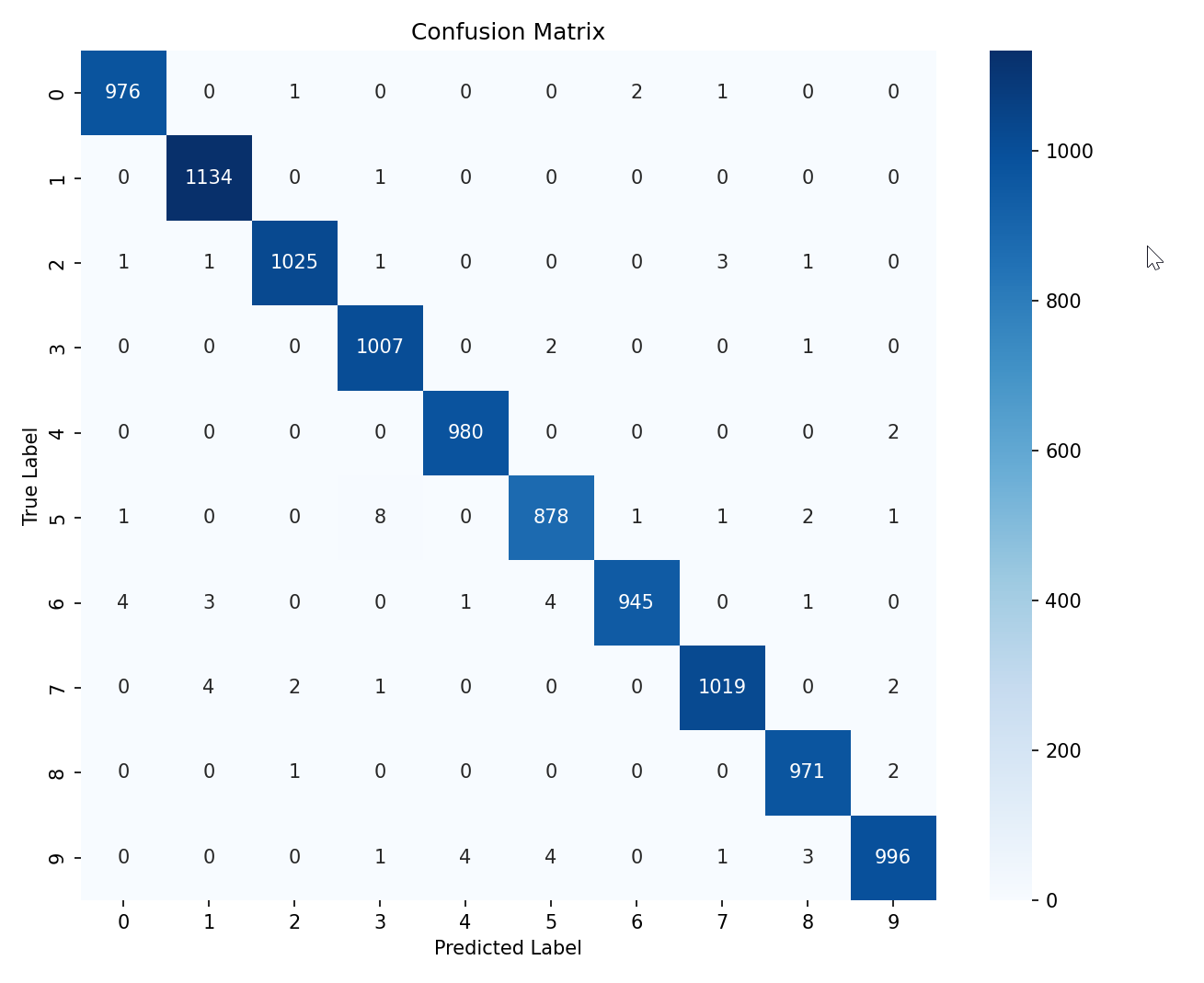
# 可视化2：混淆矩阵（修正版）
# ======================
# 获取预测结果
y_pred = model.predict(x_test)
y_pred_classes = np.argmax(y_pred, axis=1)
y_true = np.argmax(y_test, axis=1)

# 生成混淆矩阵
cm = confusion_matrix(y_true, y_pred_classes)

# 手动设置类别标签（MNIST 是 0-9）
class_names = [str(i) for i in range(10)]

# 可视化混淆矩阵
plt.figure(figsize=(10, 8))
sns.heatmap(cm, 
            annot=True,      # 在单元格中显示数值
            fmt='d',         # 数值格式为整数（适用于混淆矩阵的计数）
            cmap='Blues',    # 颜色映射（蓝色渐变）
            xticklabels=class_names,  # X轴标签（类别名称）
            yticklabels=class_names)  # Y轴标签（类别名称）
plt.title('Confusion Matrix')
plt.xlabel('Predicted Label')
plt.ylabel('True Label')
plt.show()

# ======================
# 可视化3：错误预测样本
# ======================
# 找出预测错误的样本
errors = (y_pred_classes != y_true)
error_samples = x_test[errors]
true_labels = y_true[errors]
pred_labels = y_pred_classes[errors]

# 显示前15个错误样本
plt.figure(figsize=(15, 6))
for i in range(min(15, len(error_samples))):
    plt.subplot(3, 5, i + 1)
    plt.imshow(error_samples[i].reshape(28, 28), cmap='gray')
    plt.title(f"True: {true_labels[i]}, Pred: {pred_labels[i]}")
    plt.axis('off')
plt.tight_layout()
plt.show()

# ======================
# 可视化4：特征图可视化
# ======================
# 获取第一个卷积层的输出
layer_outputs = [layer.output for layer in model.layers[:2]]
activation_model = keras.models.Model(inputs=model.input, outputs=layer_outputs)
activations = activation_model.predict(x_test[0:1])

# 显示第一卷积层的特征图
plt.figure(figsize=(12, 6))
first_layer_activation = activations[0]
for i in range(32):  # 显示前32个滤波器
    plt.subplot(4, 8, i + 1)
    plt.imshow(first_layer_activation[0, :, :, i], cmap='viridis')
    plt.axis('off')
plt.suptitle('First Convolutional Layer Activations', fontsize=16)
plt.show()

运行结果 

Epoch 15/15
422/422 [==============================] - 16s 38ms/step - loss: 0.0184 - accuracy: 0.9941 - val_loss: 0.0295 - val_accuracy: 0.9938

Training completed in 343.88 seconds
Test accuracy: 0.9931
313/313 [==============================] - 1s 2ms/step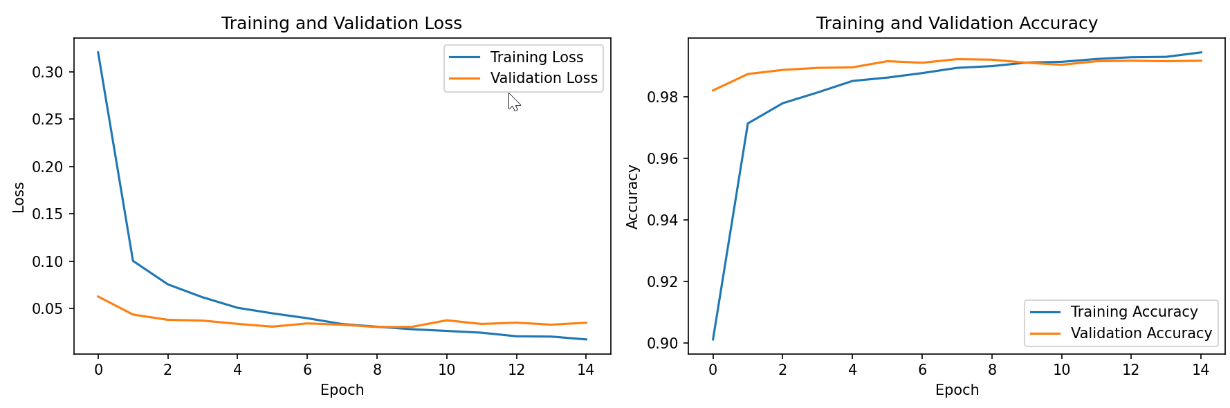

 ======================
# 3. 新增功能：随机展示20张测试集样本（调整到模型训练之后）
# ======================
def show_random_samples(model, x_test, y_test, num_samples=20):
    """显示随机测试样本及其预测结果"""
    # 确保模型已训练
    if not hasattr(model, 'layers'):
        raise ValueError("Model must be trained first")

    # 生成预测结果
    y_pred = model.predict(x_test)
    y_pred_classes = np.argmax(y_pred, axis=1)

    # 获取真实标签
    y_true = np.argmax(y_test, axis=1)

    # 随机选择样本
    sample_indices = random.sample(range(len(x_test)), num_samples)

    # 创建可视化
    plt.figure(figsize=(16, 18))
    plt.suptitle("Random Handwritten Digit Samples with Predictions\n(Green=Correct, Red=Wrong)",
                 fontsize=16, y=1.03)

    rows, cols = 4, 5
    plt.subplots_adjust(hspace=0.5, wspace=0.3)

    # 使用新版Matplotlib API
    cmap = plt.colormaps.get_cmap('RdYlGn')  # 修复弃用警告

    for i, idx in enumerate(sample_indices):
        ax = plt.subplot(rows, cols, i + 1)
        img = x_test[idx].squeeze()

        # 显示图像
        plt.imshow(img, cmap='gray')

        # 获取标签信息
        true_label = y_true[idx]
        pred_label = y_pred_classes[idx]

        # 设置标题和颜色
        color = 'green' if true_label == pred_label else 'red'
        title = f'True: {true_label}\nPred: {pred_label}'
        plt.title(title, color=color, fontsize=10, pad=8)

        plt.axis('off')

    plt.tight_layout()
    plt.show()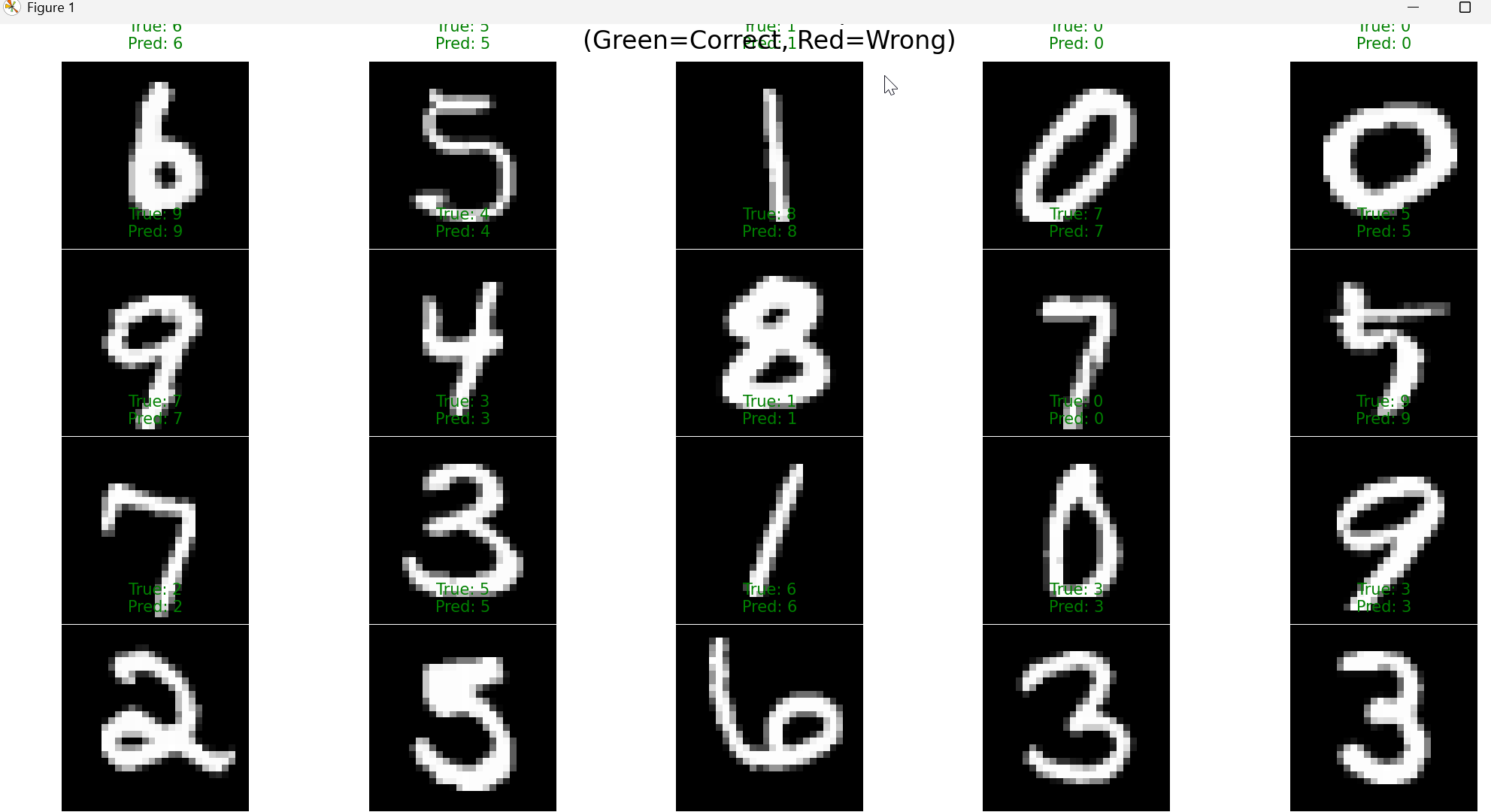

 

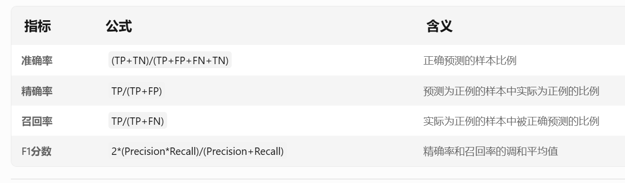
混淆矩阵基础结构

1. 矩阵布局（以二分类为例）

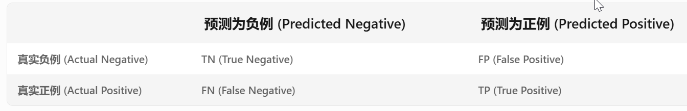
2. 关键指标计算

 

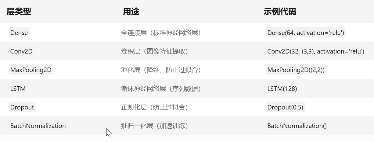
TensorFlow Keras 核心组件

1. 常用层类型

2. 构建模型的三种方式

方式1：顺序模型（Sequential API）

from tensorflow.keras import Sequential
from tensorflow.keras.layers import Dense

model = Sequential([
    Dense(128, activation='relu', input_shape=(784,)),  # 输入层
    Dense(64, activation='relu'),                       # 隐藏层
    Dense(10, activation='softmax')                     # 输出层
])

方式2：函数式API（Functional API）

from tensorflow.keras import Model
from tensorflow.keras.layers import Input, Dense

input_layer = Input(shape=(784,))
hidden = Dense(128, activation='relu')(input_layer)
output = Dense(10, activation='softmax')(hidden)
model = Model(inputs=input_layer, outputs=output)

方式3：子类化模型（Subclassing）

from tensorflow.keras import Model
from tensorflow.keras.layers import Dense

class MyModel(Model):
    def __init__(self):
        super(MyModel, self).__init__()
        self.dense1 = Dense(128, activation='relu')
        self.dense2 = Dense(10, activation='softmax')

    def call(self, inputs):
        x = self.dense1(inputs)
        return self.dense2(x)

model = MyModel()

3. 模型编译与训练

# 编译模型
model.compile(
    optimizer='adam',                 # 优化器（自动调参）
    loss='sparse_categorical_crossentropy',  # 损失函数（分类任务）
    metrics=['accuracy']              # 评估指标
)

# 训练模型
history = model.fit(
    x_train, 
    y_train,
    batch_size=32,                    # 每批样本数
    epochs=10,                        # 训练轮次
    validation_split=0.2              # 验证集比例
)