EEG代码实践：diffusion EEG——扩散模型生成EEG信号

2024/1/22：
原始EEG信号的生成说实话一直做不到让人满意的水平，之前做的MIEEG复现也迟迟没有调整到自己想要的程度，与论文中的效果还是有些差距。改换思路使用离散小波变换，用变换之后的信号做生成任务则好了许多。从大二开始一直惦记着diffusion 模型相关的EEG信号生成，开题之前去网上搜索并没有看见许多作用于EEG信号的diffusion相关论文，大多数和diffusion挂钩的论文都是做EEG视觉图像重建的。个人认为在EEG信号数据增强方面diffusion还是比较有用武之地的，因此这半个月实现了一下。在自己的原始实现结束后，尝试了使用diffuser库函数进行项目的重写，并获得了不错的成果。
博主复现项目gitee地址：(数据部分等毕业论文写完再考虑，读者可以尝试自己构建，很简单)
reference:
[1] 【大白话01】一文理清 Diffusion Model 扩散模型 | 原理图解+公式推导
[2] deepthoughts: Probabilistic Diffusion Model概率扩散模型理论与完整PyTorch代码详细解读
[3] 李宏毅 Diffusion Model
[4] hugging face 文档【diffusers】
代码部分来源：
手写部分参考reference[2]
diffuser库函数实现部分参考reference[4]
注：
文中的数学推导都是随便记录的，有错漏，想学习的话还是得看对应的视频

简单推导
一、手写实现diffusion EEG
- 1.1 导入数据
- 1.2 确定超参数的值
- 1.3 确定扩散过程任意一步的采样值
- 1.4 演示原始信号分布加噪step次后的分布
- 1.5 编写逆扩散过程高斯分布的模型
- 1.6 编写训练loss函数
- 1.7 编写逆扩散采样函数（去噪推理过程）
- 1.8 训练模型，打印loss以及中间的重构成果
二、diffusers库函数实现diffusion EEG
- 2.1 超参数配置和数据准备
- 2.2 创建训练配置
- 2.3 图像预处理
- 2.4 创建一个 UNet2DModel
- 2.5 模型测试与数据集加载
- 2.6 创建调度程序
- 2.6 训练模型
- 2.7 具体训练代码
- 2.8 启动训练
问题记录

简单推导

diffusion的前向马尔可夫过程过程如下：

$q(x_{t}|x_{t-1}) \sim \mathcal{N}(\sqrt{\alpha_{t}} x_{t-1}, 1-\alpha_{t})$
$x_{t} = \sqrt{\alpha_{t}} x_{t-1} + \sqrt{1-\alpha_{t}} \epsilon_{t-1}$
根据递推关系， $x_{t}$ 又可以表示为（下面公式仅向下递推一级）：
$x_{t} = \sqrt{\alpha_{t}} \sqrt{\alpha_{t-1}} x_{t-2} + \sqrt{\alpha_{t}} \sqrt{1-\alpha_{t-1}} \epsilon_{t-2} + \sqrt{1-\alpha_{t}} \epsilon_{t-1}$
最后可以推得 $x_{t}$ 与 $x_{0}$ 的关系：
$q(x_{t}|x_{0}) \sim \mathcal{N}(\sqrt{\overline{\alpha_{t}}} x_{0}, 1-\overline{\alpha_{t}})$
$x_{t} = \sqrt{\overline{\alpha_{t}}} x_{0} + \sqrt{1-\overline{\alpha_{t}}}\epsilon$
其中 $\overline{\alpha_{t}} = \prod_{i=1}^{t} \alpha_{i}$ ， $\epsilon$ 是一个标准正态分布的随机变量。

假设diffusion的反向过程 $q(x_{t}|x_{t-1})$ 同样服从高斯分布，那么可以得到：

$q(x_{t-1}|x_{t}) = \mathcal{N}(\mu_{t}, \sigma_{t}^{2})$

在我们的代码中，需要用神经网络进行拟合，这个过程可以简单表示为
$q_{\theta}(x_{t-1}|x_{t}) = \mathcal{N}(\mu_{\theta}(x_{t},t), \sigma_{\theta}^{2}(x_{t},t))$
拟合该分布等价于引入 $x_{0}$ ，通过贝叶斯公式可以得到：
$q(x_{t-1}|x_{t},x_{0}) = \frac{q(x_{t}|x_{t-1})q(x_{t-1}|x_{0})}{q(x_{t}|x_{0})}$
从前面，我们已经可以得到等式右边的三个高斯分布的具体状态，如下：
$q(x_{t}|x_{t-1}) \sim \mathcal{N}(\sqrt{\alpha_{t}} x_{t-1}, 1-\alpha_{t})$
$q(x_{t-1}|x_{0}) \sim \mathcal{N}(\sqrt{\overline{\alpha_{t-1}}} x_{0}, 1-\overline{\alpha_{t-1}})$
$q(x_{t}|x_{0}) \sim \mathcal{N} (\sqrt{ \overline{\alpha_{t}} x_{0}, 1-\overline{\alpha_{t}} })$

因此，我们可以得到：
$q(x_{t-1}|x_{t},x_{0}) \sim \mathcal{N}(x_{t-1} \frac{\sqrt{\alpha_{t}(1-\overline{\alpha_{t-1}})} + \sqrt{\overline{\alpha_{t-1}}}(1-\alpha_{t})}{1-\overline{\alpha_{t}}}, \frac{(1-\alpha_{t})(1-\alpha_{t-1})}{1-\overline{\alpha_{t}}})$
因为该分布的方差是固定的，所以我们只需要拟合均值即可，一开始我也不知道是怎么个拟合均值法，且看下面的代码。

一、手写实现diffusion EEG

1.1 导入数据

from data_preprocessing import *
import matplotlib.pyplot as plt
import matplotlib as mpl
import torch

mpl.rcParams['font.sans-serif'] = ['SimHei']
mpl.rcParams['axes.unicode_minus'] = False

subj = 0
task = 0
subsample = 5
epochs = 200
project_fname = './'
channel_inds = (0, 7, 9, 11, 19)

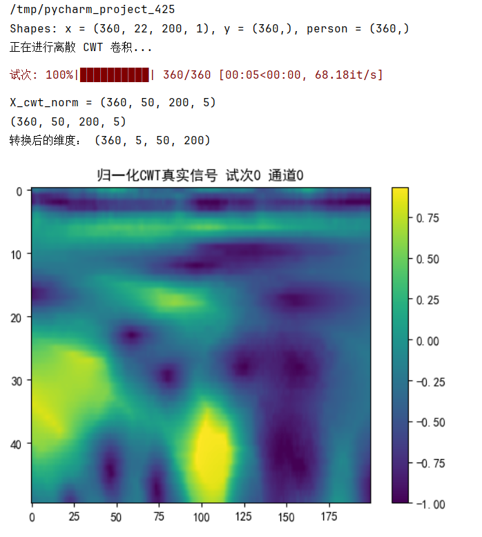
X_train_cwt_norm = WGAN_preprcessing_method(project_fname, subsample, subj, task, channel_inds)
print(X_train_cwt_norm.shape)

# 将维度转换为[trial, channel, 频段, time]
X_train_cwt_norm = X_train_cwt_norm.transpose(0, 3, 1, 2)
print("转换后的维度：", X_train_cwt_norm.shape)
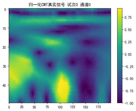
# 画出一张图
show_trial = 0
show_channel = 0
plt.figure()
plt.imshow(X_train_cwt_norm[show_trial, show_channel, :, :], aspect='auto')
plt.colorbar()
plt.title("归一化CWT真实信号 试次{} 通道{}".format(show_trial, show_channel))
plt.show()

# 转化为tensor
X_train_cwt_norm = torch.tensor(X_train_cwt_norm, dtype=torch.float32)

结果1

1.2 确定超参数的值

在之前的简略推导中，有三个关键的分布：
$q(x_{t}|x_{t-1}) \sim \mathcal{N}(\sqrt{\alpha_{t}} x_{t-1}, 1-\alpha_{t})$
$q(x_{t-1}|x_{0}) \sim \mathcal{N}(\sqrt{\overline{\alpha_{t-1}}} x_{0}, 1-\overline{\alpha_{t-1}})$
$q(x_{t}|x_{0}) \sim \mathcal{N} (\sqrt{ \overline{\alpha_{t}} x_{0}, 1-\overline{\alpha_{t}} })$

其实用 $a lp ha$ 有点便于推导的意思，但是在原版的公式中，使用的是 $\beta$ ，所以我们在这里也将 $\beta$ 定义出来，方便后续的推导。同时，我们给出了 $\beta$ 与 $\alpha$ 的关系：
$\beta = 1 - \alpha$
因此，我么可以得到类似的等价公式：
$q(x_{t}|x_{t-1}) \sim \mathcal{N}(\sqrt{\alpha_{t}} x_{t-1}, 1-\alpha_{t}) \sim \mathcal{N}(\sqrt{1-\beta_{t}} x_{t-1}, \beta_{t})$

在下面的代码中，我们会定义以下超参数：

num_step：去噪（扩散）步数
betas：每一步的 $\beta$ 值
alphas：每一步的 $\alpha$ 值
alphas_prod： $\overline{\alpha_{t}}$ 的值
alphas_prod_p： $\overline{\alpha_{t-1}}$ 的值
alpha_bar_sqrt： $\sqrt{\overline{\alpha_{t}}}$ 的值
one_minus_alpha_bar_log： $\log(1-\overline{\alpha_{t}})$ 的值
one_minus_alpha_bar_sqrt： $\sqrt{1-\overline{\alpha_{t}}}$ 的值

需要注意的是， $t$ 表示这些数组的索引，可以通过索引来获取对应的值。

# 对于step，一开始可以由beta、分布均值和方差确定
num_steps = 1500
# 指定每一步的beta
betas = torch.linspace(-6, 6, num_steps)
betas = torch.sigmoid(betas) * (0.5e-2 - 1e-5) + 1e-5

# 计算alpha、alpha_prod、alpha_prod_previous、alpha_bar_sqrt等变量的值
alphas = 1 - betas
# cumprod是累乘函数
alphas_prod = torch.cumprod(alphas, 0)
alphas_prod_p = torch.cat([torch.tensor([1]), alphas_prod[:-1]], 0)
alpha_bar_sqrt = torch.sqrt(alphas_prod)
one_minus_alpha_bar_log = torch.log(1 - alphas_prod)
one_minus_alpha_bar_sqrt = torch.sqrt(1 - alphas_prod)

# 检查shape
assert betas.shape == alphas.shape == alphas_prod.shape == alphas_prod_p.shape == alpha_bar_sqrt.shape == one_minus_alpha_bar_log.shape == one_minus_alpha_bar_sqrt.shape
print("all the same shape:", betas.shape)
# 画一张2*4的图，每个子图都是一张图
fig, axes = plt.subplots(2, 4, figsize=(40, 20))
axes = axes.flatten()
# 画图，颜色是不同的，字体
for i, (name, data) in enumerate(
        zip(["betas", "alphas", "alphas_prod", "alphas_prod_p", "alpha_bar_sqrt", "one_minus_alpha_bar_log",
             "one_minus_alpha_bar_sqrt"],
            [betas, alphas, alphas_prod, alphas_prod_p, alpha_bar_sqrt, one_minus_alpha_bar_log,
             one_minus_alpha_bar_sqrt])):
    axes[i].plot(data.numpy(), label=name, color='C{}'.format(i))
    axes[i].set_title(name, fontsize=20)
plt.show()

在这里插入图片描述

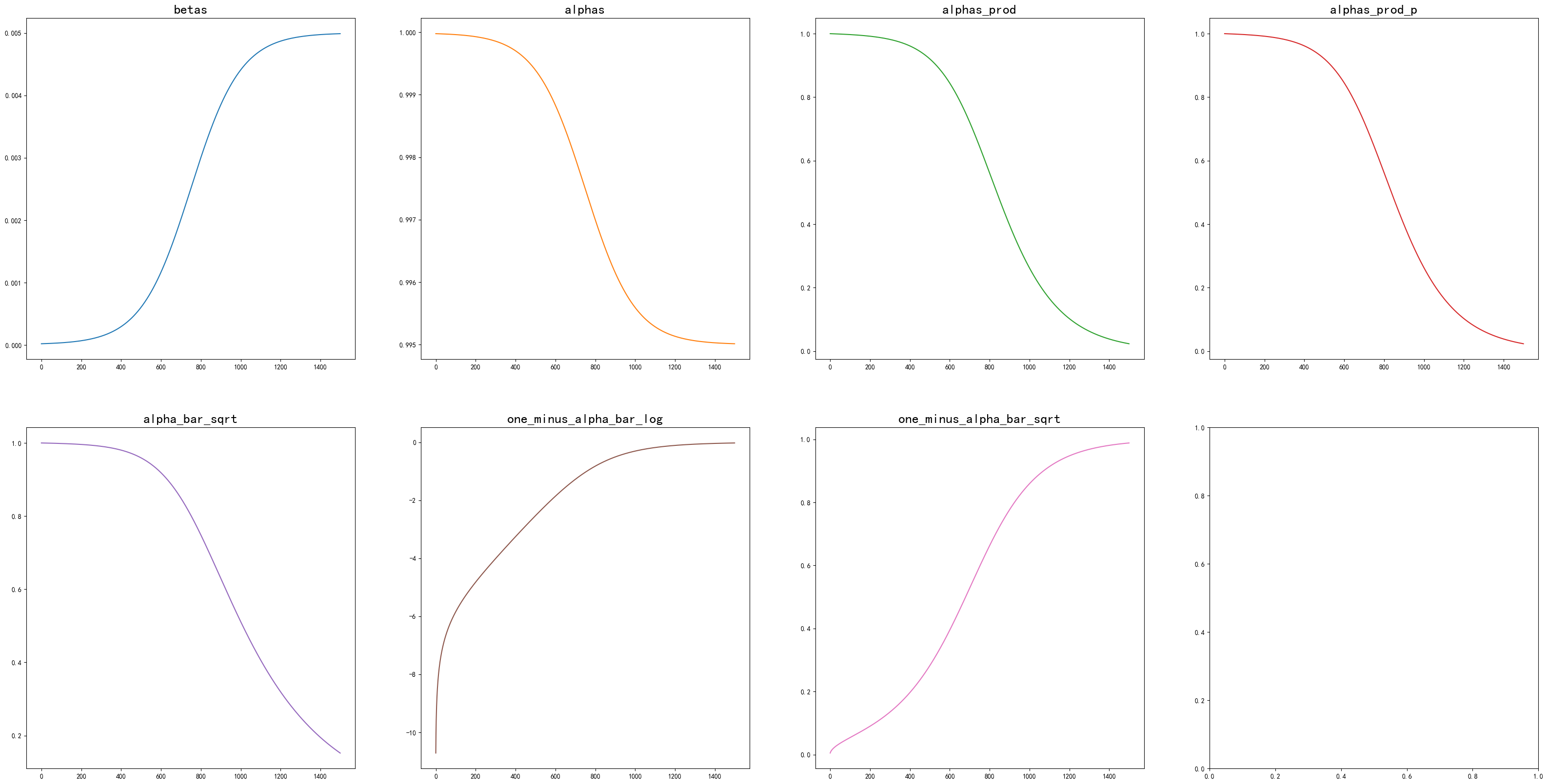
在上面的图中我们可以看到，按照我们定义的公式：
$x_{t} = \sqrt{\alpha_{t}} x_{t-1} + \sqrt{1-\alpha_{t}} \epsilon_{t-1}$
如果我们将 $\alpha_{t}$ 的值从0变化到1，那么从 $x_{0}$ 到 $x_{t}$ 的递推过程中，噪声在图像中所占的成分会逐渐增大，而原始信号的成分会逐渐减小。最后，我们可以看到，噪声的成分占据了整个信号的绝大部分。\

1.3 确定扩散过程任意一步的采样值

根据前文给出的公式：
$q(x_{t}|x_{0}) \sim \mathcal{N}(\sqrt{\overline{\alpha_{t}}} x_{0}, 1-\overline{\alpha_{t}})$
$x_{t} = \sqrt{\overline{\alpha_{t}}} x_{0} + \sqrt{1-\overline{\alpha_{t}}}\epsilon$
如果我们得到了 $x_{0}$ 的值，我们就可以计算到任意步数 $t$ 之后的 $x_{t}$ 的值，代码如下：

# 计算任意一步的采样值，基于x_0和参数重整化技巧
def q_x(x_0, t):
    return alpha_bar_sqrt[t] * x_0 + one_minus_alpha_bar_sqrt[t] * torch.randn_like(x_0)

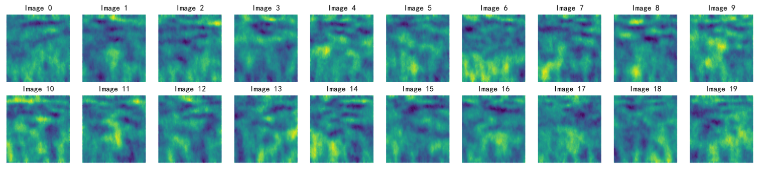
1.4 演示原始信号分布加噪step次后的分布

# 画20张图
num_shows = 20
fig, axes = plt.subplots(2, 10, figsize=(28, 6.5))
plt.rc('text', color='blue')

# 取第一个试次的信号进行加噪
x_0 = X_train_cwt_norm[0][0].squeeze()
print("原始信号的shape：", x_0.shape)

# 只用一个通道的数据测试
# 原始信号的shape： torch.Size([50, 200])
# 生成1000步内每隔num_steps//num_shows步的图
for i in range(num_shows):
    # imshow是画图函数
    j = i // 10
    k = i % 10
    # i * num_steps // num_shows是第i张图的步数
    # print("第{}步".format(i * num_steps // num_shows))
    q_i = q_x(x_0, i * num_steps // num_shows)
    axes[j, k].imshow(q_i.numpy(), aspect='auto')
    # 相似度保留两位小数
    axes[j, k].set_title("step {} 正态度：{:.2f}".format(i * num_steps // num_shows, torch.mean(q_i.pow(2)).item()))

plt.show()

# 检查最后的噪声与正态分布的相似性
q_i = q_x(x_0, num_steps - 1)
print("最后的噪声与正态分布的相似性：", torch.mean(q_i.pow(2)).item())

原始信号的shape： torch.Size([50, 200])
在这里插入图片描述
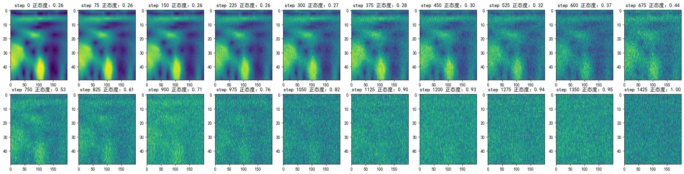
网上没有找到关于numstep的具体设置，个人感觉是numstep需要加到最后的图像为正态分布噪声为止，因此上面取了1500步，上面可以看到最后的噪声与正态分布已经很接近了。

1.5 编写逆扩散过程高斯分布的模型

之前有讲到，我们神经网络是用来拟合均值的，这里给出具体的公式：
$\mu_{\theta}(x_{t},t) = \widetilde{\mu_{t}}(x_{t}, \frac{1}{ \sqrt{\overline{\alpha_{t} }}} (x_{t}-\sqrt{1-\overline{\alpha_{t}}}\epsilon_{\theta}(x_{t})) = \frac{1}{ \sqrt{\overline{\alpha_{t} }}} (x_{t}- \frac{\beta_{t}}{ \sqrt{1-\overline{\alpha_{t}}}} \epsilon_{\theta}(x_{t}, t))$
在这个公式中， $\epsilon_{\theta}$ 就是需要我们用神经网络拟合的部分，而这个神经网络的输入是 $x_{t}$ 和 $t$ ，而神经网络输出的噪声shape应当与 $x_{t}$ 一致。

import torch
import torch.nn as nn
import torch.nn.functional as F


class ResidualConvBlock(nn.Module):
    def __init__(
            self, in_channels: int, out_channels: int, is_res: bool = False
    ) -> None:
        super().__init__()
        '''
        standard ResNet style convolutional block
        '''
        self.same_channels = in_channels == out_channels
        self.is_res = is_res
        self.conv1 = nn.Sequential(
            nn.Conv2d(in_channels, out_channels, 3, 1, 1),
            nn.BatchNorm2d(out_channels),
            nn.GELU(),
        )
        self.conv2 = nn.Sequential(
            nn.Conv2d(out_channels, out_channels, 3, 1, 1),
            nn.BatchNorm2d(out_channels),
            nn.GELU(),
        )

    def forward(self, x: torch.Tensor) -> torch.Tensor:
        if self.is_res:
            x1 = self.conv1(x)
            x2 = self.conv2(x1)
            # this adds on correct residual in case channels have increased
            if self.same_channels:
                out = x + x2
            else:
                out = x1 + x2
            return out / 1.414
        else:
            x1 = self.conv1(x)
            x2 = self.conv2(x1)
            return x2
        
class UnetDown0(nn.Module):
    def __init__(self, in_channels, out_channels):
        super(UnetDown0, self).__init__()
        '''
        process and downscale the image feature maps
        '''
        layers = [ResidualConvBlock(in_channels, out_channels), nn.MaxPool2d((1, 4))]
        self.model = nn.Sequential(*layers)

    def forward(self, x):
        return self.model(x)


class UnetDown(nn.Module):
    def __init__(self, in_channels, out_channels):
        super(UnetDown, self).__init__()
        '''
        process and downscale the image feature maps
        '''
        layers = [ResidualConvBlock(in_channels, out_channels), nn.MaxPool2d(2)]
        self.model = nn.Sequential(*layers)

    def forward(self, x):
        return self.model(x)


class UnetUp1(nn.Module):
    def __init__(self, in_channels, out_channels):
        super(UnetUp1, self).__init__()
        '''
        process and upscale the image feature maps
        '''
        layers = [
            nn.ConvTranspose2d(in_channels, out_channels, 2, 2, output_padding=(1, 1)),
            ResidualConvBlock(out_channels, out_channels),
            ResidualConvBlock(out_channels, out_channels),
        ]
        self.model = nn.Sequential(*layers)

    def forward(self, x, skip):
        x = torch.cat((x, skip), 1)
        x = self.model(x)
        return x


class UnetUp2(nn.Module):
    def __init__(self, in_channels, out_channels):
        super(UnetUp2, self).__init__()
        '''
        process and upscale the image feature maps
        '''
        layers = [
            nn.ConvTranspose2d(in_channels, out_channels, 2, 2),
            ResidualConvBlock(out_channels, out_channels),
            ResidualConvBlock(out_channels, out_channels),
        ]
        self.model = nn.Sequential(*layers)

    def forward(self, x, skip):
        x = torch.cat((x, skip), 1)
        x = self.model(x)
        return x
    
class UnetUp3(nn.Module):
    def __init__(self, in_channels, out_channels):
        super(UnetUp3, self).__init__()
        '''
        process and upscale the image feature maps
        '''
        layers = [
            nn.ConvTranspose2d(in_channels, out_channels, (1, 4), (1, 4)),
            ResidualConvBlock(out_channels, out_channels),
            ResidualConvBlock(out_channels, out_channels),
        ]
        self.model = nn.Sequential(*layers)

    def forward(self, x, skip):
        x = torch.cat((x, skip), 1)
        x = self.model(x)
        return x


class EmbedFC(nn.Module):
    def __init__(self, input_dim, emb_dim):
        super(EmbedFC, self).__init__()
        '''
        generic one layer FC NN for embedding things  
        '''
        self.input_dim = input_dim
        layers = [
            nn.Linear(input_dim, emb_dim),
            nn.GELU(),
            nn.Linear(emb_dim, emb_dim),
        ]
        self.model = nn.Sequential(*layers)

    def forward(self, x):
        x = x.view(-1, self.input_dim)
        return self.model(x)


class Unet(nn.Module):
    def __init__(self, in_channels, n_feat=256):
        super(Unet, self).__init__()

        self.in_channels = in_channels
        self.n_feat = n_feat

        self.init_conv = ResidualConvBlock(in_channels, n_feat, is_res=True)
        self.down0 = UnetDown0(n_feat, n_feat)
        self.down1 = UnetDown(n_feat, n_feat)
        self.down2 = UnetDown(n_feat, 2 * n_feat)
        # self.down3 = UnetDown(2 * n_feat, 4 * n_feat)

        self.to_vec = nn.Sequential(nn.AvgPool2d((12, 12)), nn.GELU())

        self.timeembed1 = EmbedFC(1, 2 * n_feat)
        self.timeembed2 = EmbedFC(1, 1 * n_feat)

        self.up0 = nn.Sequential(
            # nn.ConvTranspose2d(6 * n_feat, 2 * n_feat, 7, 7), # when concat temb and cemb end up w 6*n_feat
            nn.ConvTranspose2d(2 * n_feat, 2 * n_feat, (12, 12)),  # otherwise just have 2*n_feat
            nn.GroupNorm(8, 2 * n_feat),
            nn.ReLU(),
        )

        self.up1 = UnetUp1(4 * n_feat, n_feat)
        self.up2 = UnetUp2(2 * n_feat, n_feat)
        self.up3 = UnetUp3(2* n_feat, n_feat)
        self.out = nn.Sequential(
            nn.Conv2d(2 * n_feat, n_feat, 3, 1, 1),
            nn.GroupNorm(8, n_feat),
            nn.ReLU(),
            nn.Conv2d(n_feat, self.in_channels, 3, 1, 1),
        )

    def forward(self, x, t):
        '''
        输入加噪图像和对应的时间step，预测反向噪声的正态分布
        :param x: 加噪图像
        :param t: 对应step
        :return: 正态分布噪声
        '''
        x = self.init_conv(x)
        # print("x shape:", x.shape)
        down0 = self.down0(x)
        # print("down0 shape:", down0.shape)
        down1 = self.down1(down0)
        # print("down1 shape:", down1.shape)
        down2 = self.down2(down1)
        # print("down2 shape:", down2.shape)
        
        hiddenvec = self.to_vec(down2)
        # print("hiddenvec shape:", hiddenvec.shape)
        # embed time step
        # print("t shape:", t.shape)
        temb1 = self.timeembed1(t).view(-1, self.n_feat * 2, 1, 1)
        # print("temb1 shape:", temb1.shape)
        temb2 = self.timeembed2(t).view(-1, self.n_feat, 1, 1)
        # print("temb2 shape:", temb2.shape)
        temb3 = self.timeembed2(t).view(-1, self.n_feat, 1, 1)

        # 将上采样输出与step编码相加，输入到下一个上采样层
        up1 = self.up0(hiddenvec)
        # print("up1 shape:", up1.shape)
        up2 = self.up1(up1 + temb1, down2)
        # print("up2 shape:", up2.shape)
        up3 = self.up2(up2 + temb2, down1)
        # print("up3 shape:", up3.shape)
        up4 = self.up3(up3 + temb3, down0)
        # print("up4 shape:", up4.shape)
        out = self.out(torch.cat((up4, x), 1))
        return out
# 测试部分
batch_size = 4 # 可以调整
in_channels = 5  # 输入通道数
x = torch.randn(batch_size, in_channels, 50, 200)  # 输入的随机张量
t = torch.randn(batch_size, 1)  # 随机时间步

# 初始化模型
model = Unet(in_channels)
print("x shape:", x.shape)
print("t shape:", t.shape)
# 前向传播
output = model(x, t)

# 打印输出形状
print(f'输出形状: {output.shape}')

x shape: torch.Size([4, 5, 50, 200])
t shape: torch.Size([4, 1])
输出形状: torch.Size([4, 5, 50, 200])

1.6 编写训练loss函数

神经网络中的loss由以下公式计算，这里暂且省略复杂的推导过程：
$L_{simple}(\theta) := \mathbb{E}_{t,x_{0},\epsilon}[ || \epsilon - \epsilon_{\theta}( \sqrt{\overline{\alpha_{t}}} x_{0} + \sqrt{1-\overline{\alpha_{t}}}\epsilon,t ) ||^{2} ]$
这里说明一点，训练是一个马尔可夫前向的过程，属于diffusion model的真实图像到噪声的阶段，使用神经网络训练时 $x_{0}$ 是已知的，故不需要代换掉。而在下面的代码中，epsilon是一个标准正态分布的随机变量，我们可以通过torch.randn_like(x_0)来生成。
这里讲一下我是如何在直觉上理解该公式的：

我们代码中定义的噪声epislon是在diffusion的前向过程中作用在 $x_0$ 上通过公式将其按照 $t$ 转变为 $x_t$ 的噪声，我们神经网络的目标就是通过 $x_t$ 和 $t$ 来预测出这个噪声，所以我们的loss就是预测的噪声与真实噪声的差值。我们需要让神经网络拟合这个噪声的原因是，加噪和去噪在直觉上是一个逆过程（虽然数学的推导并没有这么简单），只要拿到 $x_0$ 走 $t$ 步的噪声（当t到一个很大的程度，比如我们的nums_steps时， $x_t$ （这时候也可以称为 $x_T$ ）近似为正态分布），那么我们就可以通过这个加噪过程的噪声，以正态分布为起点来做一个逆过程的去噪，以此来得到新样本。

我一开始也对“为什么需要随机取t”存在疑问，而这本质上是没有理解我们需要预测的噪声是哪种噪声。其实从前面的公式看：
$x_{t} = \sqrt{\alpha_{t}} x_{t-1} + \sqrt{1-\alpha_{t}} \epsilon_{t-1}$
然后递推得到：
$x_{t} = \sqrt{\overline{\alpha_{t}}} x_{0} + \sqrt{1-\overline{\alpha_{t}}}\epsilon$
$x_0$ 到 $x_t$ 是可以一步到位的，并且我们最终的逆向过程需要的也是这个一步到位的噪声（就是在上一小节的公式末尾中我们提到的 $\epsilon_{\theta}(x_{t}, t)$ ），而不是中间一步一步的噪声，所以我们需要随机取t来提高训练效率，但是个人感觉不随机也没有太大问题。

def diffusion_loss_fn(model, x_0, alphas_bar_sqrt, one_minus_alpha_bar_sqrt, n_steps, device):
    """
    对任意时刻的t进行采样计算来训练loss
    """
    # 为batch_size 随机采样一个时刻t，为了提高训练效率，保证t不重复
    t = torch.randint(0, n_steps, size=(batch_size//2,), device=device)  # 指定设备
    t = torch.cat([t, n_steps-1-t], dim=0)
    t = t.unsqueeze(-1)
    
    # x_0的系数
    a = alphas_bar_sqrt[t].to(device)  # 确保在同一设备上
    # epislon的系数
    aml = one_minus_alpha_bar_sqrt[t].to(device)  # 确保在同一设备上
    # 生成随机噪声
    epsilon = torch.randn_like(x_0, device=device)  # 确保噪声也在同一设备上
    # 构建模型输入
    x_t = a.view(-1, 1, 1, 1) * x_0 + aml.view(-1, 1, 1, 1) * epsilon
    x_t = x_t.to(dtype=torch.float32)
    t = t.to(dtype=torch.float32)  # 确保 t 在同一设备上
    # 导入模型，得到t时刻的随机噪声预测值
    output = model(x_t, t)
    
    # 与真实噪声一起计算误差，求平均值
    return (epsilon - output).square().mean()

1.7 编写逆扩散采样函数（去噪推理过程）

在简单推导的最后，提到了这样一个公式作为逆扩散的噪声：
$q(x_{t-1}|x_{t},x_{0}) \sim \mathcal{N}(x_{t-1} \frac{\sqrt{\alpha_{t}(1-\overline{\alpha_{t-1}})} + \sqrt{\overline{\alpha_{t-1}}}(1-\alpha_{t})}{1-\overline{\alpha_{t}}}, \frac{(1-\alpha_{t})(1-\alpha_{t-1})}{1-\overline{\alpha_{t}}})$

下面的p_sample函数中，涉及到了之前我们提过的均值拟合：
$\mu_{\theta}(x_{t},t) = \widetilde{\mu_{t}}(x_{t}, \frac{1}{ \sqrt{\overline{\alpha_{t} }}} (x_{t}-\sqrt{1-\overline{\alpha_{t}}}\epsilon_{\theta}(x_{t})) = \frac{1}{ \sqrt{\overline{\alpha_{t} }}} (x_{t}- \frac{\beta_{t}}{ \sqrt{1-\overline{\alpha_{t}}}} \epsilon_{\theta}(x_{t}, t))$
该公式提到了从 $x_{t}$ 逆扩散至 $x_{t-1}$ 过程中的均值规定，与此同时，方差不涉及到任何一个样本和未知量，是一个确定的值。在下面的代码中，我们将不断使用p_sample函数得到每一步逆扩散的均值然后得到逆扩散噪声，直至逆扩散至 $x_{0}$ 。

def p_sample_loop(model, shape, n_steps, betas, one_minus_alpha_bar_sqrt):
    """
    从x_T逆扩散至x_{T-1}、x_{T-2}、...、x_0
    """
    cur_x = torch.randn(shape)  # 将张量初始化到指定设备
    x_seq = [cur_x]
    
    for i in reversed(range(n_steps)):
        cur_x = p_sample(model, cur_x, i, betas, one_minus_alpha_bar_sqrt)
        x_seq.append(cur_x)
    
    return x_seq

def p_sample(model, x, t, betas, one_minus_alpha_bar_sqrt):
    """
    从x_T采样至t时刻的样本
    """
    t = torch.tensor([t])

    # 确保 betas 和 one_minus_alpha_bar_sqrt 在正确设备上
    
    # 使用 t 索引 betas 和 one_minus_alpha_bar_sqrt
    coeff = betas[t] / one_minus_alpha_bar_sqrt[t]  # 确保 betas 和 one_minus_alpha_bar_sqrt 在相同设备上
    with torch.no_grad():
        eps_theta = model(x.to(device), t.to(dtype=torch.float32).to(device))  # 计算模型输出
    mean = (1 / (1 - betas[t].cpu())) * (x.cpu() - coeff.cpu() * eps_theta.cpu())  # 计算均值
    
    z = torch.randn_like(x)  # 确保噪声张量 z 在相同的设备上
    sigma_t = betas[t].sqrt()  # 计算标准差
    
    sample = mean + sigma_t.cpu() * z  # 生成样本
    return sample

1.8 训练模型，打印loss以及中间的重构成果

接下来应该没什么需要解释的东西了

import torch
import matplotlib.pyplot as plt
from torch.utils.data import DataLoader

# 构建一个参数平滑器
class EMA():
    def __init__(self, mu=0.01):
        self.mu = mu
        self.shadow = {}
        
    def register(self, name, val):
        self.shadow[name] = val.clone()
        
    def __call__(self, name, x):
        assert name in self.shadow
        new_average = (1.0 - self.mu) * self.shadow[name] + self.mu * x
        self.shadow[name] = new_average.clone()
        return new_average

print("training...")

batch_size = 18
dataloaders = torch.utils.data.DataLoader(X_train_cwt_norm, batch_size=batch_size, shuffle=True)
num_epoch = 1000
plt.rc('text', color='blue')

# 使用 CUDA，如果可用的话
device = torch.device("cuda" if torch.cuda.is_available() else "cpu")

# 将模型移到 GPU
model = Unet(in_channels).to(device)
optimizer = torch.optim.Adam(model.parameters(), lr=1e-4)

# EMA实例
ema = EMA()

# 假设 alpha_bar_sqrt, one_minus_alpha_bar_sqrt 已经在设备上
alpha_bar_sqrt = alpha_bar_sqrt.to(device)  # 确保在同一设备上
one_minus_alpha_bar_sqrt = one_minus_alpha_bar_sqrt.to(device)  # 确保在同一设备上
betas = betas.to(device)  # betas 也需要在同一设备上

from tqdm import tqdm

# 在外层循环中初始化进度条
with tqdm(range(num_epoch), desc='Epochs') as pbar_epoch:
    for t in pbar_epoch:
        # 在每个 epoch 内部循环
        for idx, batch_x in enumerate(dataloaders):
            batch_x = batch_x.to(device)  # 将 batch_x 移动到正确设备上
            
            optimizer.zero_grad()
        
            # 计算损失并进行反向传播
            loss = diffusion_loss_fn(model, batch_x, alpha_bar_sqrt, one_minus_alpha_bar_sqrt, num_steps, device)
            loss.backward()
            
            # 梯度裁剪
            torch.nn.utils.clip_grad_norm_(model.parameters(), 1.0)
            
            # 更新参数
            optimizer.step()
        
        # 每次 epoch 完成后更新外层进度条
        pbar_epoch.set_postfix({'Epoch': t + 1})

        # 更新EMA
        """for name, param in model.named_parameters():
            if param.requires_grad:
                ema(name, param.data)

        # 更新进度条信息，显示当前批次的损失
        pbar.set_postfix(loss=loss.item())"""
        
        # 每100个epoch打印一次
        if (t + 1) % 100 == 0:
            print("Epoch {} Loss: {:.4f}".format(t + 1, loss.item()))
            
            # 生成图像并显示
            x_seq = p_sample_loop(model, batch_x.shape, num_steps, betas, one_minus_alpha_bar_sqrt)
            fig, axes = plt.subplots(1, 10, figsize=(28, 3.2))
            
            # nums_steps//10步生成一张图
            for i in range(10):
                x_pic = x_seq[i * num_steps // 10][0][0].squeeze().detach().cpu().numpy()
                axes[i].imshow(x_pic, aspect='auto')
                axes[i].set_title("epoch {} step {}".format(t + 1, i * num_steps // 10))
            plt.show()

"""
50 * 200
x shape: torch.Size([8, 5, 50, 200])
t shape: torch.Size([8, 1])
x shape: torch.Size([8, 256, 50, 200])
down0 shape: torch.Size([8, 256, 50, 50])
down1 shape: torch.Size([8, 256, 25, 25])
down2 shape: torch.Size([8, 512, 12, 12])
hiddenvec shape: torch.Size([8, 512, 1, 1])
temb1 shape: torch.Size([8, 512, 1, 1])
temb2 shape: torch.Size([8, 256, 1, 1])
up1 shape: torch.Size([8, 512, 12, 12])
up2 shape: torch.Size([8, 256, 25, 25])
up3 shape: torch.Size([8, 256, 50, 50])
up4 shape: torch.Size([8, 256, 50, 200])
输出形状: torch.Size([8, 5, 50, 200])
"""

这代码折腾了很久，之前出现了to.(cuda)加错位置导致爆显存的问题——深度学习做了两三年第一次碰到爆显存。解决该问题之后，笔电3060还是爆显存。迫不得已去autodl租了张4090跑，结果也没快到哪里去——初步判断是我的神经网络的某几层参数量过大导致的，这个Unet可能需要之后再优化。

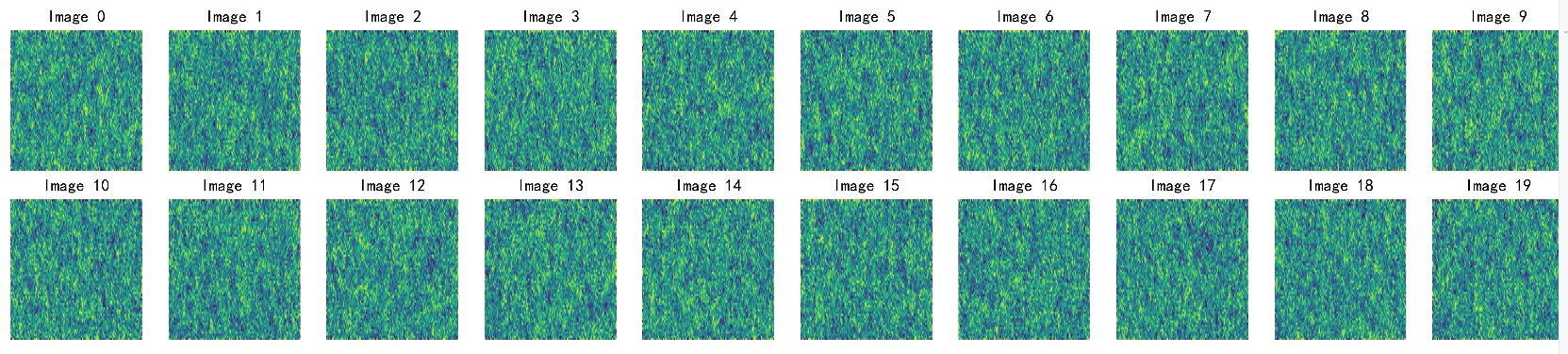
最后跑了500轮出来效果一般，差不多跟前面加噪100层差不多，原来是想跑2000轮的，但是程序无error提示直接退出了。查看了一下AutoPanel，内存的使用大小随着训练的进行呈现阶段性提升，可能代码在内存方面存在一定的问题。加之跑一轮——尤其是生成图片样本的推理时间长的离谱，因此简单贴一下500epoch的结果。

在这里插入图片描述

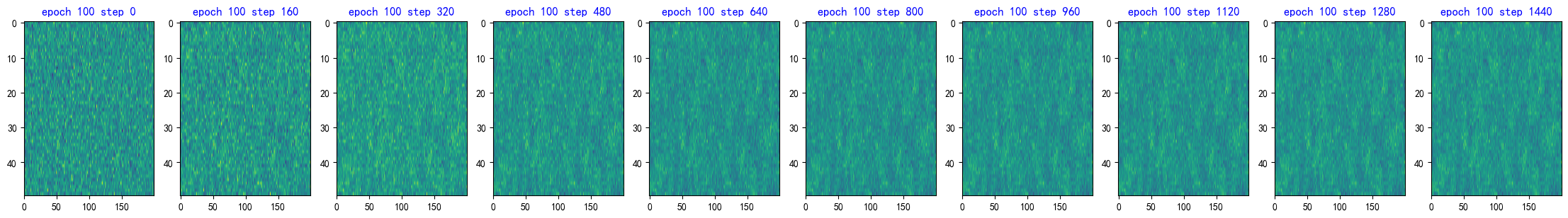
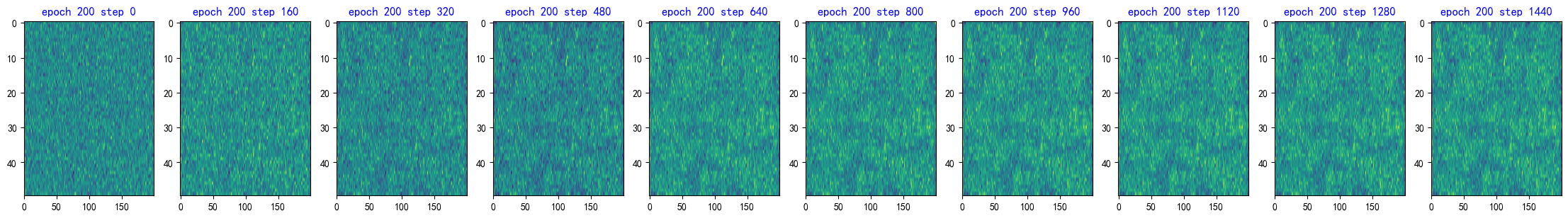
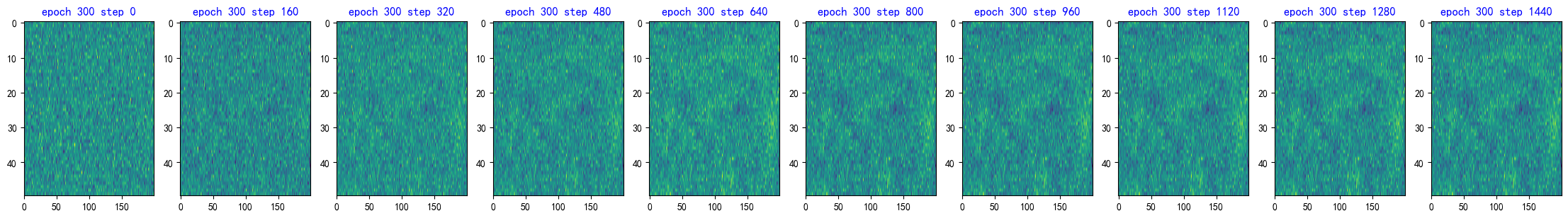
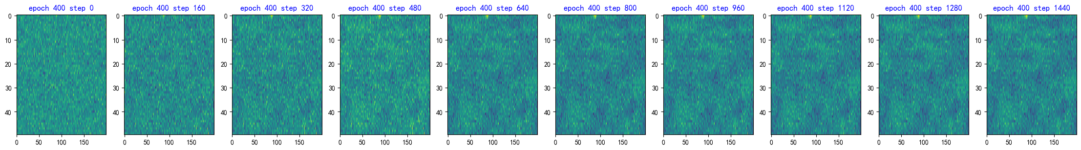
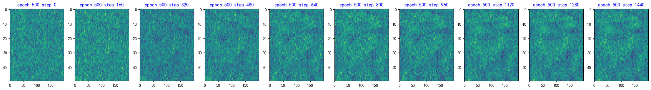
其实结果也算有模有样，如果跑2000轮效果估计还会好一点。

二、diffusers库函数实现diffusion EEG

手写部分大概花了我两天左右，调试和debug差不多又花了一天，结果跑出来一般。diffusers的实现基本完全参考了官方文档和部分源码，只花了我一下午的时间就做到了不错的成果，果然还是要依靠前人的智慧。

详细的提示等官方文档里都有，这里不多说了。

2.1 超参数配置和数据准备

from data_preprocessing import *
import matplotlib.pyplot as plt
import matplotlib as mpl
import torch

mpl.rcParams['font.sans-serif'] = ['SimHei']
mpl.rcParams['axes.unicode_minus'] = False

subj = 0
task = 0
subsample = 5
project_fname = './'
pic_dir = os.path.join('./model_pic/DDPM/', 'suj' + str(subj), 'task' + str(task))
output_dir = './model_checkpoints/ckpt-DDPN/'

print("图片输出文件夹：", pic_dir)
print("模型输出文件夹：", output_dir)

os.makedirs(pic_dir, exist_ok=True)
    
channel_inds = (0, 7, 9, 11, 19)

图片输出文件夹： ./model_pic/DDPM/suj0/task0
模型输出文件夹： ./model_checkpoints/ckpt-DDPN/

X_train_cwt_norm = WGAN_preprcessing_method(project_fname, subsample, subj, task, channel_inds)
print(X_train_cwt_norm.shape)

# 将维度转换为[trial, channel, 频段, time]
X_train_cwt_norm = X_train_cwt_norm.transpose(0, 3, 1, 2)
# 将第三个维度
print("转换后的维度：", X_train_cwt_norm.shape)
# 画出一张图
show_trial = 0
show_channel = 0
plt.figure()
plt.imshow(X_train_cwt_norm[show_trial, show_channel, :, :], aspect='auto')
plt.colorbar()
plt.title("归一化CWT真实信号 试次{} 通道{}".format(show_trial, show_channel))
plt.show()

# 转化为tensor
X_train_cwt_norm = torch.tensor(X_train_cwt_norm, dtype=torch.float32)

/tmp/pycharm_project_425
Shapes: x = (360, 22, 200, 1), y = (360,), person = (360,)
正在进行离散 CWT 卷积…
试次: 100%|██████████| 360/360 [00:04<00:00, 82.69it/s]
X_cwt_norm = (360, 50, 200, 5)
(360, 50, 200, 5)
转换后的维度： (360, 5, 50, 200)
在这里插入图片描述

2.2 创建训练配置

为方便起见，创建一个 TrainingConfig 类，其中包含训练超参数。如果需要使用自己的数据集，更改image_size等相关参数即可。

from dataclasses import dataclass

@dataclass
class TrainingConfig:
    # 图像尺寸
    image_size = (64, 256)
    # 训练批次大小
    train_batch_size = 36
    # 评估批次大小 
    eval_batch_size = 36
    # 训练轮数
    num_epochs = 50
    # 梯度累积步数（累计几次梯度更新一次参数）
    gradient_accumulation_steps = 1
    # 学习率
    learning_rate = 1e-4
    # 学习率衰减
    lr_warmup_steps = 500
    
    save_image_epochs = 10
    save_model_epochs = 30
    
    mixed_precision = "no"  # `no` for float32, `fp16` for automatic mixed precision
    output_dir = output_dir
    # 是否上传模型到HF Hub
    push_to_hub = False  # whether to upload the saved model to the HF Hub
    hub_model_id = "hibiscus/test_model"  # the name of the repository to create on the HF Hub
    hub_private_repo = None
    overwrite_output_dir = True  # overwrite the old model when re-running the notebook
    seed = 42
    
config = TrainingConfig()

2.3 图像预处理

diffusers库中规定，输入Unet的图像边长必须为64及其倍数，故这里扩张了一下。

# 预处理保证图像尺寸正确
from torchvision import transforms

preprocess = transforms.Compose([
    transforms.Resize(config.image_size),
])

def transform_image(img):
    return preprocess(img)

X_train_cwt_norm = transform_image(X_train_cwt_norm)
print("转换后的维度：", X_train_cwt_norm.shape)

转换后的维度： torch.Size([360, 5, 64, 256])

2.4 创建一个 UNet2DModel

from diffusers import UNet2DModel

model = UNet2DModel(
    sample_size=config.image_size,  # the target image resolution
    in_channels=5,  # the number of input channels, 3 for RGB images
    out_channels=5,  # the number of output channels
    layers_per_block=2,  # how many ResNet layers to use per UNet block
    block_out_channels=(128, 128, 256, 256, 512, 512),  # the number of output channels for each UNet block
    down_block_types=(
        "DownBlock2D",  # a regular ResNet downsampling block
        "DownBlock2D",
        "DownBlock2D",
        "DownBlock2D",
        "AttnDownBlock2D",  # a ResNet downsampling block with spatial self-attention
        "DownBlock2D",
    ),
    up_block_types=(
        "UpBlock2D",  # a regular ResNet upsampling block
        "AttnUpBlock2D",  # a ResNet upsampling block with spatial self-attention
        "UpBlock2D",
        "UpBlock2D",
        "UpBlock2D",
        "UpBlock2D",
    ),
)

2.5 模型测试与数据集加载

# 测试输入输出
# 选取采样通道
sample_channel = 0
sample_image = X_train_cwt_norm[0].unsqueeze(0)
print("输入图像维度：", sample_image.shape)

print("Output shape:", model(sample_image, timestep=0).sample.shape)

输入图像维度： torch.Size([1, 5, 64, 256])
Output shape: torch.Size([1, 5, 64, 256])

import torch
from torch.utils.data import DataLoader, Dataset

train_dataloader = DataLoader(X_train_cwt_norm, batch_size=config.train_batch_size, shuffle=True)

2.6 创建调度程序

测试得到num_train_timesteps的合适值，查看加噪后的图像分布

import torch
from diffusers import DDPMScheduler

test_noise_steps = 100

noise_scheduler = DDPMScheduler(num_train_timesteps=1000)
noise = torch.randn(sample_image.shape)
timesteps = torch.LongTensor([test_noise_steps])
noisy_image = noise_scheduler.add_noise(sample_image, noise, timesteps)

# 每加噪100步的图像，画出一张图，一共10张
fig, axs = plt.subplots(1, 10, figsize=(20, 2))
for i in range(0, 10):
    timesteps = torch.LongTensor([test_noise_steps*i])
    noisy_image = noise_scheduler.add_noise(sample_image, noise, timesteps)
    axs[i].imshow(noisy_image[0, 0, :, :].detach().numpy(), aspect='auto')

    axs[i].axis("off")
    axs[i].set_title(f"Step {i * 100}")

在这里插入图片描述
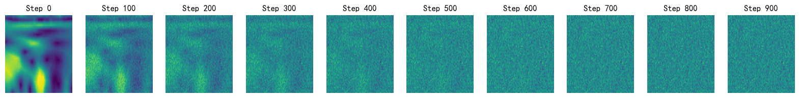
diffusers库中的加噪函数显然比自己手写的方式更快达到正态噪声的效果，不知道采取了什么方案。

2.6 训练模型

创建优化器和学习率调度程序：

from diffusers.optimization import get_cosine_schedule_with_warmup

optimizer = torch.optim.AdamW(model.parameters(), lr=config.learning_rate)
lr_scheduler = get_cosine_schedule_with_warmup(
    optimizer=optimizer,
    num_warmup_steps=config.lr_warmup_steps,
    num_training_steps=(len(train_dataloader) * config.num_epochs),
)

构造评估模型的方法，使用 DDPMPipeline 生成一批样本图像并将其保存为图片。这里有个比较大的坑，DDPMpipeline默认的输出为一个PIL image list且支支持3通道，需要手动加一下output_type="np.array"才能输出多通道的np.array类型数据，jupyter运行的时候这里报错居然不显示，因此花了一段较长的时间找bug。

from diffusers import DDPMPipeline
from diffusers.utils import make_image_grid
import os

def evaluate(config, epoch, pipeline):
    # 从随机噪声中生成一些图像（这是反向扩散过程）。
    # 默认的管道输出类型是 `List[torch.Tensor]`
    # 取sample_channel来展示
    # print("生成图像......")

    images = pipeline(
        batch_size=config.eval_batch_size,
        generator=torch.Generator(device='cpu').manual_seed(config.seed),  # 使用单独的 torch 生成器来避免回绕主训练循环的随机状态
        output_type="np.array",
    ).images

    print("生成图像维度：", images.shape)
    # (batch, height, width, channel)

    # 将生成的eval_batch_size个图像拼接成一张大图
    pig, ax = plt.subplots(2, 10, figsize=(20, 4))
    for i in range(2):
        for j in range(10):
            ax[i, j].imshow(images[i * 10 + j, :, :, sample_channel], aspect='auto')
            ax[i, j].axis("off")
            ax[i, j].set_title(f"Image {i * 10 + j}")

    plt.savefig(f"{pic_dir}/{epoch:04d}.png", dpi=400)
    plt.close()

2.7 具体训练代码

from accelerate import Accelerator
import torch.nn.functional as F
from huggingface_hub import create_repo, upload_folder
from tqdm.auto import tqdm
from pathlib import Path
import os

def train_loop(config, model, noise_scheduler, optimizer, train_dataloader, lr_scheduler):
    # Initialize accelerator and tensorboard logging
    accelerator = Accelerator(
        mixed_precision=config.mixed_precision,
        gradient_accumulation_steps=config.gradient_accumulation_steps,
        log_with="tensorboard",
        project_dir=os.path.join(config.output_dir, "logs"),
    )
    if accelerator.is_main_process:
        if config.output_dir is not None:
            os.makedirs(config.output_dir, exist_ok=True)
        if config.push_to_hub:
            repo_id = create_repo(
                repo_id=config.hub_model_id or Path(config.output_dir).name, exist_ok=True
            ).repo_id
        accelerator.init_trackers("train_example")

    # Prepare everything
    # There is no specific order to remember, you just need to unpack the
    # objects in the same order you gave them to the prepare method.
    model, optimizer, train_dataloader, lr_scheduler = accelerator.prepare(
        model, optimizer, train_dataloader, lr_scheduler
    )

    global_step = 0

    # Now you train the model
    for epoch in range(config.num_epochs):
        progress_bar = tqdm(total=len(train_dataloader), disable=not accelerator.is_local_main_process)
        progress_bar.set_description(f"Epoch {epoch}")

        for step, batch in enumerate(train_dataloader):
            clean_images = batch
            # Sample noise to add to the images
            noise = torch.randn(clean_images.shape, device=clean_images.device)
            bs = clean_images.shape[0]

            # Sample a random timestep for each image
            timesteps = torch.randint(
                0, noise_scheduler.config.num_train_timesteps, (bs,), device=clean_images.device,
                dtype=torch.int64
            )

            # Add noise to the clean images according to the noise magnitude at each timestep
            # (this is the forward diffusion process)
            noisy_images = noise_scheduler.add_noise(clean_images, noise, timesteps)

            with accelerator.accumulate(model):
                # Predict the noise residual
                noise_pred = model(noisy_images, timesteps, return_dict=False)[0]
                loss = F.mse_loss(noise_pred, noise)
                accelerator.backward(loss)

                if accelerator.sync_gradients:
                    accelerator.clip_grad_norm_(model.parameters(), 1.0)
                optimizer.step()
                lr_scheduler.step()
                optimizer.zero_grad()

            progress_bar.update(1)
            logs = {"loss": loss.detach().item(), "lr": lr_scheduler.get_last_lr()[0], "step": global_step}
            progress_bar.set_postfix(**logs)
            accelerator.log(logs, step=global_step)
            global_step += 1

        # After each epoch you optionally sample some demo images with evaluate() and save the model
        if accelerator.is_main_process:
            pipeline = DDPMPipeline(unet=accelerator.unwrap_model(model), scheduler=noise_scheduler)

            if (epoch + 1) % config.save_image_epochs == 0 or epoch == config.num_epochs - 1:
                evaluate(config, epoch, pipeline)

            if (epoch + 1) % config.save_model_epochs == 0 or epoch == config.num_epochs - 1:
                if config.push_to_hub:
                    upload_folder(
                        repo_id=repo_id,
                        folder_path=config.output_dir,
                        commit_message=f"Epoch {epoch}",
                        ignore_patterns=["step_*", "epoch_*"],
                    )
                else:
                    pipeline.save_pretrained(config.output_dir)

2.8 启动训练

from accelerate import notebook_launcher

args = (config, model, noise_scheduler, optimizer, train_dataloader, lr_scheduler)

notebook_launcher(train_loop, args, num_processes=1)

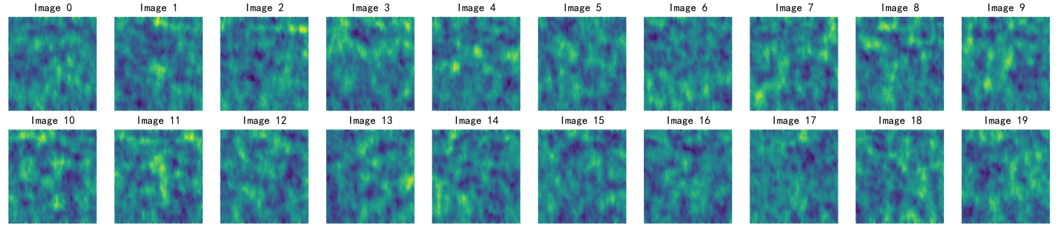
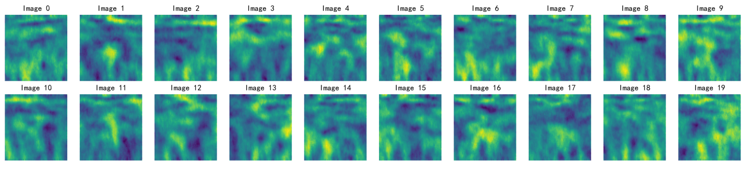
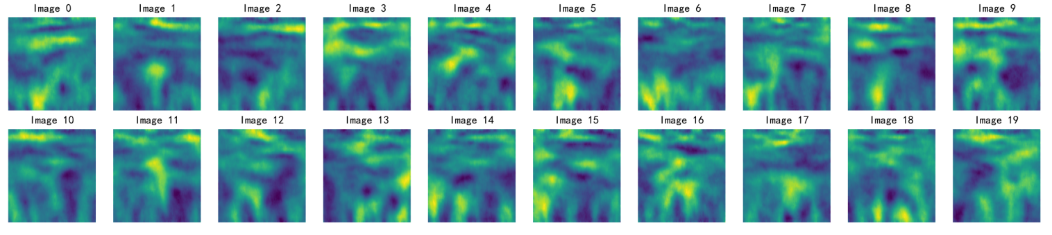
按照上面的config，一共训练了50轮，每10轮生成一批图像，效果远比手写500epoch生成的图像质量更好，训练得到结果如下：

在这里插入图片描述

问题记录

在跑手写实现模型的时候遇到了显存爆炸但是gpu无占用的问题，具体表现如下：

在这里插入图片描述
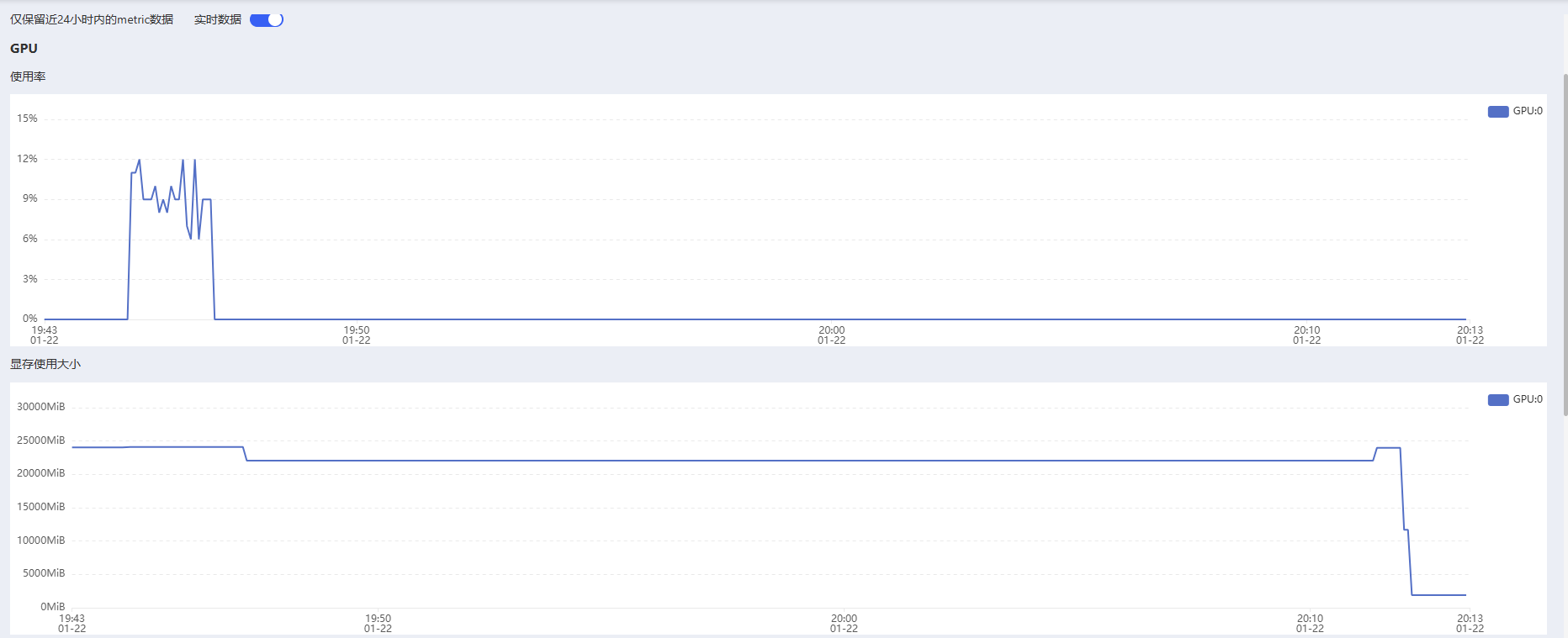
后面的显存回落是解决问题后的成果。比较令人费解的是，根据网络上大火说的，nvidia-smi 命令执行之后，应当会列出当前所有使用进程所使用的GPU memory大小，而我这里显示的却全是占用0MiB，这误导了我很久。

问题的具体影响有：
在问题出现之前batch_size=64可以正常运行，但是问题出现后改成更小的batch_size也会立刻报显存爆炸的error。
在这里插入图片描述
我是使用本机的pycharm上的jupyter使用ssh连接autodl上实例来跑代码的。原来以为是僵尸进程占用了gpu，但是后来排查发现不存在僵尸进程。最后确认问题的原因还是出在jupyter上：