1. 前言

在第 21 章中，我介绍了 Elasticsearch 的读优化，但你是否曾疑惑：如何在上线前判断查询的耗时？
在第 22 章中，我提到可以通过 Explain API查看文档所在的索引，但这个 API 的功能是否仅限于此？
本章将深入探讨 Profile API 和 Explain API，帮助你了解如何在上线前识别查询问题，以及 Elasticsearch 是如何计算文档评分的。

2. Profile API - 查询优化

Profile API 用于查看 DSL 性能瓶颈。只需要添加 "profile": true 即可查看 DSL 的执行性能。

2.1 Profile API 简单介绍

接下来，我将通过一个简单的例子，带大家了解其使用

写入测试数据

POST _bulk
{ "index" : { "_index" : "test_23", "_id" : "1" } }
{"name": "hello elasticsearch","tag": "happy,love,easy", "platform": 1}
{ "index" : { "_index" : "test_23", "_id" : "2" } }
{"name": "hello java","tag": "platform,performance,easy", "platform": 2}
{ "index" : { "_index" : "test_23", "_id" : "3" } }
{"name": "hello go","tag": "platform,performance,easy", "platform": 3}

使用 profile API

GET test_23/_search?human=true
{
  "profile": true, 
  "query": {
    "bool": {
      "must": [
        {
          "multi_match": {
            "query": "hello",
            "fields": ["name", "tag"]
          } 
        }
      ],
      "filter": [
        {
          "range": {
            "platform": {
              "gte": 0,
              "lte": 20
            }
          }
        }
      ]
    }
  }
}

Profile API 的输出包含以下几个信息

• shards(Array) ：每个分片上的执行情况
• shards.searches(Array) ：每个查询都换转换为 Lucene 中处理的搜索实体
• shards.searches.query(Array) ：执行的各个 Lucene 查询breakdown
• shards.searches.query.breakdown(Object) ：Lucene 索引中各种执行方法的计时及执行次数
• shards.searches.query.children(Array) : query 的每个子查询，结构上看是嵌套的
• shards.searches.rewrite_time(Value) : 将 ES 查询转换为 Lucene 最佳查询
• shards.searches.collector(Array) ：负责从文档中收集匹配的结果
• shards.aggregations(Array) ：聚合查询信息
• shards.aggregations.breakdown(Object) ：Lucene 索引中各种执行方法的计时及执行次数
• shards.aggregations.children(Array) : query 的每个子查询，结构上看是嵌套的

我们一般关心只每个子查询所花费的时间，即 time_in_nanos 字段。我们一般不关心 breakdown 所展示的底层方法执行时间。因为我们控制不了，我们只能控制我们传给 ES 的查询语句。

例如，上面的例子，所返回的信息，只需要关注每个子查询所花费的时间，针对每个查询去做优化即可。

{
  "profile": {
    "shards": [
      {
        "searches": {
          "query": [
            {
              "type": "BooleanQuery",
              "description": "+(tag:hello | name:hello) #platform:[0 TO 20]",
              "time_in_nanos": 744800,
              "children": [
                {
                  "type": "DisjunctionMaxQuery",
                  "description": "(tag:hello | name:hello)",
                  "time_in_nanos": 352300,
                  "children": [
                    {
                      "type": "TermQuery",
                      "description": "tag:hello",
                      "time_in_nanos": 40000
                    },
                    {
                      "type": "TermQuery",
                      "description": "name:hello",
                      "time_in_nanos": 117100
                    }
                  ]
                },
                {
                  "type": "IndexOrDocValuesQuery",
                  "description": "platform:[0 TO 20]",
                  "time_in_nanos": 67200
                }
              ]
            }
          ]
        }
      }
    ]
  }
}

2.2 查询结果图形化

上面的例子，我们介绍了使用 API 的方式去查看 DSL 的性能。但实际上 kibana 有提供图形化界面，让我们更直观的查看 DSL 性能。

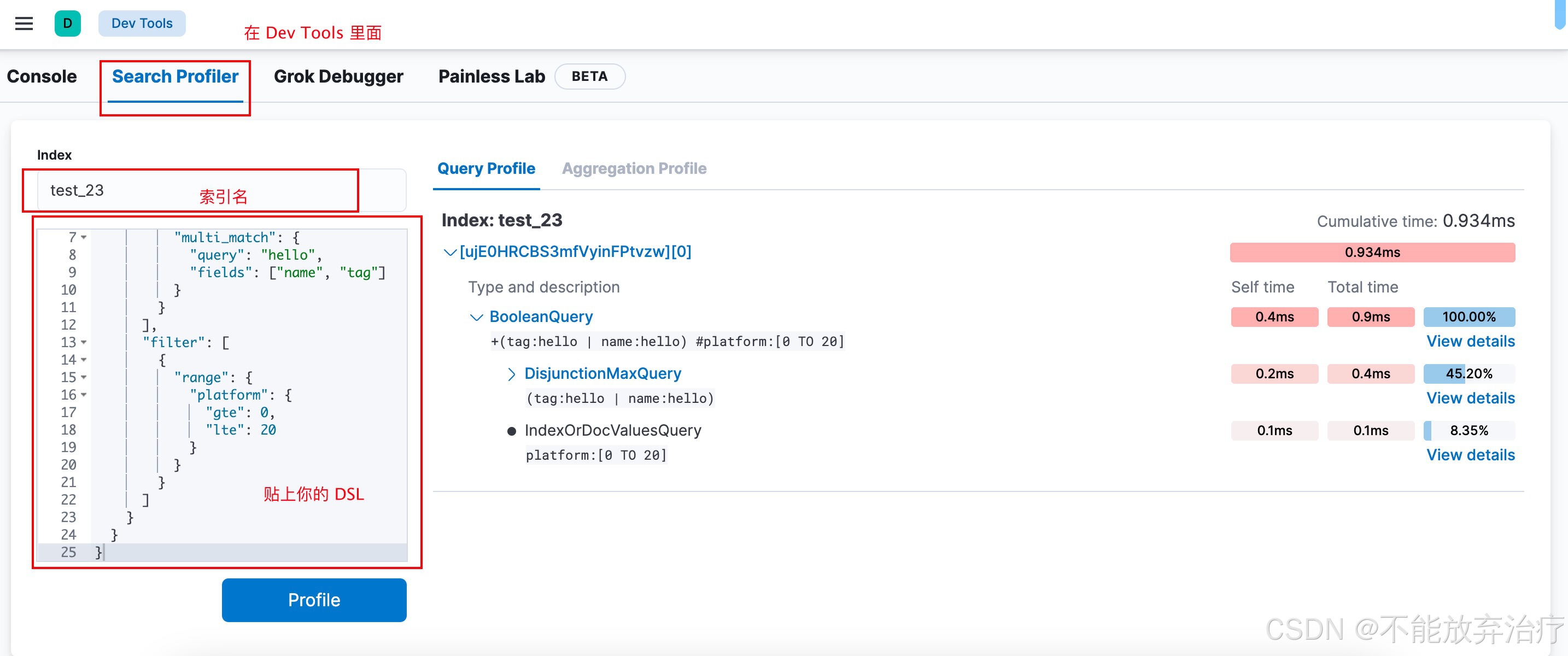
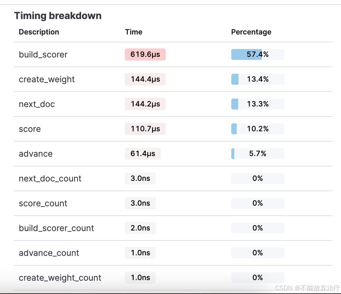
点击 view details 显示的就是 breakdown 的内容

2.3 Profile 注意事项

1. 避免在 ES 高负载情况下执行 Profile API, 因为 Profile API 会增加查询的开销，可能会加重集群负载
2. Profile API 不测量网络延迟、请求在队列中花费的时间或在协调节点上合并碎片响应所花费的时间。

3. Explain API - 解释查询

Explain API 用于理解文档相关性评分，开发中用得到的场景不多。在 22 章，有简单提到过使用方式，这里重新复习一遍。

GET test_23/_search
{
  "explain": true,
   "query": {
    "bool": {
      "must": [
        {
          "multi_match": {
            "query": "hello",
            "fields": ["name", "tag"]
          } 
        }
      ],
      "filter": [
        {
            "term": {
            "platform": 1
          }
        }
      ]
    }
  }
}

接下来，我会带大家通过 explain 输出的内容，再复习一次 22 章中所讲到的 BM25 相关性评分的内容。

上述查询，输出如下

{
  "value": 0.13353139,
  "description": "sum of:",
  "details": [
    {
      "value": 0.13353139,
      "description": "max of:",
      "details": [
        {   ----- ①
          "value": 0.13353139,
          "description": "score(freq=1.0), computed as boost * idf * tf from:",     
          "details": [
            {      ----- ②
              "value": 2.2,
              "description": "boost",
              "details": []
            },
            {    ----- ③
              "value": 0.13353139,
              "description": "idf, computed as log(1 + (N - n + 0.5) / (n + 0.5)) from:",      
              "details": [
                {
                  "value": 3,
                  "description": "n, number of documents containing term",
                  "details": []
                },
                {
                  "value": 3,
                  "description": "N, total number of documents with field",
                  "details": []
                }
              ]
            },
            {   ----- ④
              "value": 0.45454544,
              "description": "tf, computed as freq / (freq + k1 * (1 - b + b * dl / avgdl)) from:",
              "details": [
                {
                  "value": 1,
                  "description": "freq, occurrences of term within document",
                  "details": []
                },
                {
                  "value": 1.2,
                  "description": "k1, term saturation parameter",
                  "details": []
                },
                {
                  "value": 0.75,
                  "description": "b, length normalization parameter",
                  "details": []
                },
                {
                  "value": 2,
                  "description": "dl, length of field",
                  "details": []
                },
                {
                  "value": 2,
                  "description": "avgdl, average length of field",
                  "details": []
                }
              ]
            }
          ]
        }
      ]
    }
  ]
}

• ①: 告诉我们计算公式为：score(freq=1.0), computed as boost * idf * tf from:
• ②：告诉我们 boost 的取值为 2.2
• ③：告诉我们 IDF 计算公式为：idf, computed as log(1 + (N - n + 0.5) / (n + 0.5)) from:。
  该公式等同于 $ln(1+\frac{(docCount-f(q_i)+0.5)}{f(q_i)+0.5})$。其中 $docCount=N$，$f(q_i)=n$
• ④：告诉我们 tf 计算公式为：tf, computed as freq / (freq + k1 * (1 - b + b * dl / avgdl)) from:
  该公式等同于 $\frac{f(q_i,D)\ast (k1+1)}{f(q_i,D)+k1\ast (1-b+b\ast \frac{fieldLen}{avgFieldLen})}$。其中 $f(q_i,D)=freq$

一般很少关注这个，简单做下了解即可。