1.算法概述

我们使用11或13维特征向量表示图像中的每个像素。两个特征用于表示像素之间的空间关系；由图像尺寸规格化的x和y像素坐标。对于灰度图像，一个特征是低通表示，它捕获平均图像强度。（低通r、g和b平面用于彩色图像）。我们使用8个特征来表示纹理信息，使用对一组定向过滤器的响应。最后，利用主成分分析法对特征空间进行降维。详细说明如下。

二、a、平均灰度（和颜色信息）

我们使用中值滤波从图像中提取平均灰度和颜色信息。我们使用了一个11像素宽的中值滤波器，因为它充分抑制了小尺度纹理信息，同时仍能很好地保留轮廓和边界信息。对于彩色图像，我们对每个颜色平面应用中值过滤器。图2a和2b显示了使用的低通颜色和灰度特征。

二、b、纹理特征提取

为了提取纹理特征，我们考虑与人类前注意纹理识别机制进行类比[9]。该模型包括（1）与一组偶数对称线性滤波器进行卷积，然后进行半波校正，以给出一组V1简单细胞的响应建模输出，然后（2）在空间中定位的抑制，当相同或附近位置存在强响应时，会抑制弱响应，最后（3）纹理边界检测。

我们使用高斯差分（DOG）和偏移高斯差分滤波器（DOOG）作为线性滤波器。使用的DOG过滤器对斑点区域和使用的DOOG过滤器作出响应，对不同方向的障碍区域作出响应。我们使用两种不同的DOG滤波器来检测两个不同的斑点区域和6个不同的方向DOOG过滤器的数量。过滤器如图3所示。纹理图像对单个过滤器的响应如图4所示。请注意，与其他纹理分割方法不同，我们只使用单个尺度的过滤器（8像素宽）。我们这样做是因为在较高的比例下，纹理区域不会受到模糊瑕疵的影响，因此我们选择不使用这些区域进行纹理合成。在这一步之后，我们采用全波整流，而不是半波整流。半波校正用于复制纹理区域和它们的负片之间的区分。然而，在我们使用的小范围内，这种区分并不十分必要，我们更喜欢使用全波区分。

为了复制步骤（2）和（3），我们不使用抑制和纹理边界检测，而是使用一个简单的9像素宽中值滤波器。众所周知，中值滤波器在强响应存在时抑制弱响应，并且仍然保持边界信息。因此，中值滤波器在一个步骤中实现了步骤（2）和（3）。

我们基于以下对细分的洞察力进行研究。考虑图6a所示的图像及其纹理特征（使用斑点过滤器），如图6b所示。我们可以直观地将4b分割为两个区域，有纹理和无纹理。现在考虑图6c，它显示了4b的随机抽样子集。仍然可以定义轮廓并对图像进行分割，类似于4b中的分割。在这个分割之后，如果我们考虑所有剩余的点，那么它们可以在这个初始分割的基础上被分类为有纹理的或无纹理的。根据这一见解，我们推导出以下算法。

图像被分割成不同的条形、斑点和模糊区域后，我们应用一种简单的基于规则的启发式算法将区域分类为潜在的模糊伪影及其对应的源区域（纹理未丢失的区域）。这种启发式应该具有低错误识别的特点。作为这一过程的第一步，我们将上一节中的每个片段确定为“有纹理”和“无纹理”。

2.仿真效果预览

matlab2022a仿真

3.MATLAB部分代码预览

disp('Preprocessing...');tic;
% Preprocess all
[allfeatures, rDims, cDims, depth] = preprocfast(img);
[samples,olddimensions] = size(allfeatures);
gallfeatures = allfeatures;
 
% Combine all texture features to use for later thresholding
% Also save all low pass features for later adjacency processing
if depth == 1
    texturefeature = max(allfeatures(:,4:11), [], 2);
    lowpassfeature = allfeatures(:,3);
    lowpassimage = reshape(lowpassfeature, [cDims rDims])';
else
    texturefeature = max(allfeatures(:,6:13), [], 2);
    lowpassfeature = allfeatures(:,3:5);
    lowpassimage(:,:,1) = reshape(lowpassfeature(:,1), [cDims rDims])';
    lowpassimage(:,:,2) = reshape(lowpassfeature(:,2), [cDims rDims])';
    lowpassimage(:,:,3) = reshape(lowpassfeature(:,3), [cDims rDims])';
end
textures = reshape(texturefeature, [cDims rDims])';
% Principle component based dimensionality reduction of all features
allfeatures = pca(allfeatures, 0.05); 
% Choose 10% of samples randomly and save in DATASET
[samples, dimensions] = size(allfeatures);
% We work on ~WORKSAMPLES pixels. If the image has less we use all pixels. 
% If not then the appropriate portion of pixels is randomly selected.
worksamples = samples/10;
if worksamples < 10000
    worksamples = 10000;
end
if samples < worksamples
    worksamples = samples;
end
choose = rand([samples 1]); choose = choose < (worksamples/samples); 
dataset = zeros([sum(choose), dimensions]);
dataset(1:sum(choose),:) = allfeatures(find(choose),:); % find(choose) returns array where choose is non zero
disp('Preprocessing done.');t = toc; totalt = totalt + t;
disp(['     Original dimensions: ' int2str(olddimensions)]);
disp(['     Reduced dimensions by PCA: ' int2str(dimensions)]);
disp(['     Image has ' int2str(rDims * cDims) ' pixels.']);
disp(['     Using only ' int2str(size(dataset,1)) ' pixels.']);
disp(['Elapsed time: ' num2str(t)]);
disp(' ');
% SEGMENTATION
%   1. k-means (on sampled image)
%   2. Use centroids to classify remaining points
%   3. Classify spatially disconnected regions as separate regions
% Segmentation Step 1. 
%   k-means (on sampled image)
% Compute k-means on randomly sampled points
disp('Computing k-means...');tic;
% Set number of clusters heuristically.
k = round((rDims*cDims)/(100*100)); k = max(k,8); k = min(k,16);
% Uncomment this line when MATLAB k-means unavailable
%[centroids,esq,map] = kmeanlbg(dataset,k);
[map, centroids] = kmeans(dataset, k);  % Calculate k-means (use MATLAB k-mean
disp('k-means done.');t = toc; totalt = totalt + t;
disp(['     Number of clusters: ' int2str(k)]);
disp(['Elapsed time: ' num2str(t)]);
disp(' ');
% Segmentation Step 2. 
%   Use centroids to classify the remaining points
disp('Using centroids to classify all points...');tic;
globsegimage = postproc(centroids, allfeatures, rDims, cDims);   % Use centroids to classify all points
% Segmentation Step 3.
%   Classify spatially disconnected regions as separate regions
globsegimage = medfilt2(globsegimage, [3 3], 'symmetric');
globsegimage = imfill(globsegimage);
region_count = max(max(globsegimage));
count = 1; newglobsegimage = zeros(size(globsegimage));
for i = 1:region_count
    region = (globsegimage == i);
    [bw, num] = bwlabel(region);
    for j = 1:num
        newglobsegimage = newglobsegimage + count*(bw == j);
        count = count + 1;
    end
end
oldglobsegimage = globsegimage;
globsegimage = newglobsegimage;
disp('Classification done.');t = toc; totalt = totalt + t;
disp(['Elapsed time: ' num2str(t)]);
disp(' ');
% DISPLAY IMAGES
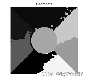
% Display segments
%figure(1), imshow(globsegimage./max(max(globsegimage)));
figure(1), imshow(label2rgb(globsegimage, 'gray'));
title('Segments');
% Calculate boundary of segments
BW = edge(globsegimage,'sobel', 0);
% Superimpose boundary on original image
iout = img;
if (depth == 1) % Gray image, so use color lines
    iout(:,:,1) = iout;
    iout(:,:,2) = iout(:,:,1);
    iout(:,:,3) = iout(:,:,1);
    iout(:,:,2) = min(iout(:,:,2) + BW, 1.0);
    iout(:,:,3) = min(iout(:,:,3) + BW, 1.0);
else            % RGB image, so use white lines
    iout(:,:,1) = min(iout(:,:,1) + BW, 1.0);
    iout(:,:,2) = min(iout(:,:,2) + BW, 1.0);
    iout(:,:,3) = min(iout(:,:,3) + BW, 1.0);
end
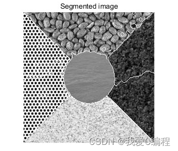
% Display image and segments
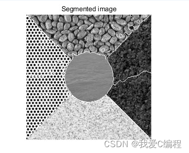
figure(2), imshow(iout);
title('Segmented image');
% POST PROCESSING AND AUTOMATIC SELECTION OF SOURCE AND TARGET REGIONS
%   1. Find overall textured region using Otsu's method (MATLAB graythresh)
%   2. Save each region and region boundary separately and note index of
%      textured regions
%   3. For each textured region, find all adjacent untextured regions and
%      save in adjacency matrix. Regions having a significant common border
%      are considered adjacent.
%   4. Find similarity between textured and adjacent untextured regions
%      using average gray level matching (average color matching). For each
%      textured region, drop those adjacent regions which don't match in
%      gray level.
disp('Post-processing and automatically selecting source and target regions...');tic;
% POSTPROC Step 1
threshold = graythresh(rescalegray(textures));
bwtexture = textures > threshold;
tex_edges = edge(bwtexture, 'sobel', 0);
figure(3),
if depth == 1
    imshow(min(img + tex_edges, 1));
else
    imshow(min(img + cat(3, tex_edges, tex_edges, tex_edges), 1));
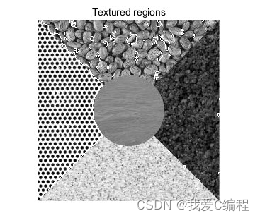
end
title('Textured regions');
% POSTPROC Step 2
% Save each region in a dimension
% Save each region boundary in a dimension
% For each region which can be classified as a textured region store index
region_count = max(max(globsegimage));
number_tex_regions = 1; tex_list = [];
for region_number = 1:region_count 
    bwregion = (globsegimage == region_number);
    
    regions(:,:,region_number) = bwregion; % Save all regions
    region_boundaries(:,:,region_number) = edge(bwregion, 'sobel', 0);
    if ( (sum(sum(bwregion.*bwtexture))/sum(sum(bwregion)) > 0.75) && sum(sum(bwregion)) > (32*32) )
        tex_list = [tex_list region_number];
        number_tex_regions = number_tex_regions + 1;
    end
end
number_tex_regions = number_tex_regions - 1;
% POSTPROC Step 3
% Find texture region adjacency and create an adjacency matrix
for i = 1:size(tex_list, 2)
    for j = 1:region_count
        if (tex_list(i) ~= j)
            boundary_overlap = sum(sum( region_boundaries(:,:,tex_list(i)).*region_boundaries(:,:,j) ));
            boundary_total_length = sum(sum( region_boundaries(:,:,tex_list(i)))) + sum(sum(region_boundaries(:,:,j)));
            if (boundary_overlap/boundary_total_length > 0) % If overlap is at least 20% of total boundary length
                region_adjacency(i,j) = boundary_overlap;     % accept it as a boundary
            end
        end
    end
end
% EXPERIMENTAL
region_adj_hard_coded = (region_adjacency - 0.2*repmat(mean(region_adjacency,2), [1 size(region_adjacency,2)])) > 0;
% Copy adjacency into another variable and remove all references to 
% textured regions from the adjacency matrix.
region_output = region_adj_hard_coded;
for tex_count = 1:size(tex_list, 2)
    region_output(:,tex_list(tex_count)) = 0;
end
% POSTPROC Step 4
% Find similarity between textured and adjacent untextured regions
% (This could be changed to a chi-squared distance between histograms of
%  textLP and adjacent by commenting out required code, and uncommenting 
%  other code, as directed in the source)
% For all textured regions find and save average brightness
for tex_count = 1:size(tex_list, 2)
    if depth == 1 
        tex_avg_bright(tex_count) = sum(sum(regions(:,:,tex_list(tex_count)).*lowpassimage)) ...
                         / sum(sum(regions(:,:,tex_list(tex_count))));
        % Comment previous and uncomment next line(s) to use histogram
        % processing   
        %tex_hist{tex_count} = histproc(regions(:,:,tex_list(tex_count)), lowpassimage);
    else
        tex_avg_bright(1,tex_count) = sum(sum(regions(:,:,tex_list(tex_count)).*lowpassimage(:,:,1))) ...
                                / sum(sum(regions(:,:,tex_list(tex_count))));
        tex_avg_bright(2,tex_count) = sum(sum(regions(:,:,tex_list(tex_count)).*lowpassimage(:,:,2))) ...
                                / sum(sum(regions(:,:,tex_list(tex_count))));
        tex_avg_bright(3,tex_count) = sum(sum(regions(:,:,tex_list(tex_count)).*lowpassimage(:,:,3))) ...
                                / sum(sum(regions(:,:,tex_list(tex_count))));
        % Comment previous and uncomment next line(s) to use histogram
        % processing        
        % tex_hist{tex_count} = histproc(regions(:,:,tex_list(tex_count)), lowpassimage);
    end
end
% For all textured regions, consider each non-textured region and update
% adjacency matrix. Keep the relationship if gray levels (colors) are similar and 
% drop if the gray levels (colors) don't match.
for tex_count = 1:size(tex_list, 2) % For all textured regions
    for adj_reg_count = 1:size(region_adj_hard_coded, 2)
        if (region_adj_hard_coded(tex_count, adj_reg_count) > 0)
            if depth == 1
                region_avg_bright = sum(sum(regions(:,:,adj_reg_count).*lowpassimage)) ...
                                    / sum(sum(regions(:,:,adj_reg_count)));
                % Comment previous and uncomment next line(s) to use histogram
                % processing   
                % region_hist = histproc(regions(:,:,adj_reg_count), lowpassimage);
            else
                region_avg_bright(1) = sum(sum(regions(:,:,adj_reg_count).*lowpassimage(:,:,1))) ...
                                    / sum(sum(regions(:,:,adj_reg_count)));
                region_avg_bright(2) = sum(sum(regions(:,:,adj_reg_count).*lowpassimage(:,:,2))) ...
                                    / sum(sum(regions(:,:,adj_reg_count)));
                region_avg_bright(3) = sum(sum(regions(:,:,adj_reg_count).*lowpassimage(:,:,3))) ...
                                    / sum(sum(regions(:,:,adj_reg_count)));
                % Comment previous and uncomment next line(s) to use histogram
                % processing                                   
                % region_hist = histproc(regions(:,:,adj_reg_count), lowpassimage);
            end
            
            if depth == 1
                if abs(tex_avg_bright(tex_count) - region_avg_bright) > 0.2 % Highly similar
                    region_output(tex_count, adj_reg_count) = 0;
                end
                % Comment previous and uncomment next line(s) to use histogram
                % processing                   
%                 if chisq(tex_hist{tex_count}, region_hist) > 0.4
%                     chisq(tex_hist{tex_count}, region_hist)
%                     region_output(tex_count, adj_reg_count) = 0;
%                 end
            else
                if mean(abs(tex_avg_bright(:,tex_count) - region_avg_bright')) > 0.2
                    region_output(tex_count, adj_reg_count) = 0;
                end
                % Comment previous and uncomment next line(s) to use histogram
                % processing                   
%                 thist = tex_hist{tex_count};
%                 chisq(thist(:,1),region_hist(:,1))
%                 chisq(thist(:,2),region_hist(:,2))
%                 chisq(thist(:,3),region_hist(:,3))
%                 t = 0.9;
%                 if (chisq(thist(:,1),region_hist(:,1)) > t) || ...
%                    (chisq(thist(:,2),region_hist(:,2)) > t) || ...
%                    (chisq(thist(:,3),region_hist(:,3)) > t)
%                     region_output(tex_count, adj_reg_count) = 0;
%                 end
            end         
        end
    end
end
disp('Post-processing done.'); t = toc; totalt = totalt + t;
disp(['Elapsed time: ' num2str(t)]);
disp(' ');
disp(['Total time elapsed: ' int2str(floor(totalt/60)) ' minutes ' int2str(mod(totalt,60)) ' seconds.']);
% DISPLAY IMAGES
% Display source and target regions.
if depth == 1
    imgs = zeros([rDims cDims size(tex_list,2)]);
    for tex_count = 1:size(tex_list, 2)
        if (sum(region_output(tex_count,:) > 0)) % If we have target patches
            imgs(:,:,tex_count) = regions(:,:,tex_list(tex_count)).*img; % Save that source patch
            for i = 1:size(region_output, 2) % For each region
                if (region_output(tex_count, i) > 0)    % which is connected to that source patch
                    imgs(:,:,tex_count) = imgs(:,:,tex_count) + 0.5*regions(:,:,i).*img; % Save the target patch
                end
            end
            figure, imshow(min(imgs(:,:,tex_count) + BW, 1));
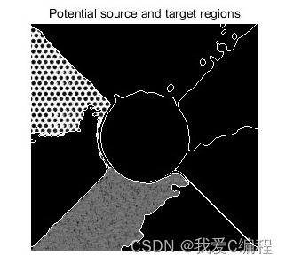
            ggg{tex_count} = min(imgs(:,:,tex_count) + BW, 1);
            title('Potential source and target regions');
        end
    end
else % depth == 3 
    count = 1;
    for tex_count = 1:size(tex_list, 2)
        if (sum(region_output(tex_count,:) > 0)) % If we have target patches
            tmp(:,:,1) = regions(:,:,tex_list(tex_count)).*img(:,:,1);
            tmp(:,:,2) = regions(:,:,tex_list(tex_count)).*img(:,:,2);
            tmp(:,:,3) = regions(:,:,tex_list(tex_count)).*img(:,:,3);
            imgs{count} = tmp;
            for i = 1:size(region_output, 2) % For each region
                if (region_output(tex_count, i) > 0)    % which is connected to that source patch
                    tmp(:,:,1) = 0.5*regions(:,:,i).*img(:,:,1);
                    tmp(:,:,2) = 0.5*regions(:,:,i).*img(:,:,2);
                    tmp(:,:,3) = 0.5*regions(:,:,i).*img(:,:,3);
                    imgs{count} = imgs{count} + tmp;
                end
            end
            figure, imshow(min(imgs{count} + cat(3,BW,BW,BW), 1));
            ggg{count} = min(imgs{count} + cat(3,BW,BW,BW), 1);
            title('Potential source and target regions');
            count = count+1;
        end
    end
end
A11