《------往期经典推荐------》
一、【100个深度学习实战项目】【链接】,持续更新~~
二、机器学习实战专栏【链接】,已更新31期,欢迎关注,持续更新中~~
三、深度学习【Pytorch】专栏【链接】
四、【Stable Diffusion绘画系列】专栏【链接】
五、YOLOv8改进专栏【链接】,持续更新中~~
六、YOLO性能对比专栏【链接】,持续更新中~
《------正文------》
目录
- 1.原始数据分析
- 1.1 查看数据基本信息
- 1.2 绘图查看数据分布
- 2.数据预处理
- 2.1 数据特征编码与on-hot处理
- 3.模型训练与调优
- 3.1 数据划分
- 3.2 模型训练调优
- 3.3 模型评估
1.原始数据分析
1.1 查看数据基本信息
#import libraries
import numpy as np
import matplotlib.pyplot as plt
import pandas as pd
#Load Data
data = pd.read_csv('/kaggle/input/brain-tumor-dataset/brain_tumor_dataset.csv')
#insights from data
data.head()
| Tumor Type | Location | Size (cm) | Grade | Patient Age | Gender | |
|---|---|---|---|---|---|---|
| 0 | Oligodendroglioma | Occipital Lobe | 9.23 | I | 48 | Female |
| 1 | Ependymoma | Occipital Lobe | 0.87 | II | 47 | Male |
| 2 | Meningioma | Occipital Lobe | 2.33 | II | 12 | Female |
| 3 | Ependymoma | Occipital Lobe | 1.45 | III | 38 | Female |
| 4 | Ependymoma | Brainstem | 6.45 | I | 35 | Female |
data.shape
(1000, 6)
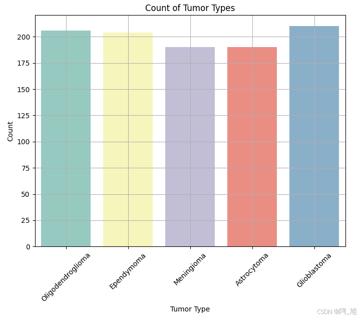
脑肿瘤的类型查看,共5种。
data['Tumor Type'].unique()
array(['Oligodendroglioma', 'Ependymoma', 'Meningioma', 'Astrocytoma',
       'Glioblastoma'], dtype=object)
data.describe()
| Size (cm) | Patient Age | |
|---|---|---|
| count | 1000.000000 | 1000.000000 |
| mean | 5.221500 | 43.519000 |
| std | 2.827318 | 25.005818 |
| min | 0.510000 | 1.000000 |
| 25% | 2.760000 | 22.000000 |
| 50% | 5.265000 | 43.000000 |
| 75% | 7.692500 | 65.000000 |
| max | 10.000000 | 89.000000 |
#Percentage of missing values in the dataset
missing_percentage = (data.isnull().sum() / len(data)) * 100
print(missing_percentage)
Tumor Type     0.0
Location       0.0
Size (cm)      0.0
Grade          0.0
Patient Age    0.0
Gender         0.0
dtype: float64
没有缺失数据
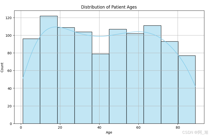
1.2 绘图查看数据分布
import seaborn as sns

plt.figure(figsize=(10, 6))
sns.histplot(data['Patient Age'], bins=10, kde=True, color='skyblue')
plt.title('Distribution of Patient Ages')
plt.xlabel('Age')
plt.ylabel('Count')
plt.grid(True)
plt.show()
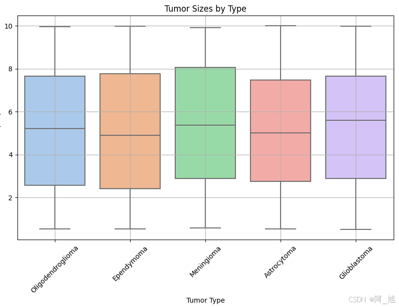
plt.figure(figsize=(10, 6))
sns.boxplot(x='Tumor Type', y='Size (cm)', data=data, palette='pastel')
plt.title('Tumor Sizes by Type')
plt.xticks(rotation=45)
plt.xlabel('Tumor Type')
plt.ylabel('Size (cm)')
plt.grid(True)
plt.show()
plt.figure(figsize=(8, 6))
sns.countplot(x='Tumor Type', data=data, palette='Set3')
plt.title('Count of Tumor Types')
plt.xlabel('Tumor Type')
plt.ylabel('Count')
plt.xticks(rotation=45)
plt.grid(True)
plt.show()
plt.figure(figsize=(10, 6))
sns.scatterplot(x='Size (cm)', y='Patient Age', hue='Tumor Type', data=data, palette='Set2', s=100)
plt.title('Tumor Sizes vs. Patient Ages')
plt.xlabel('Size (cm)')
plt.ylabel('Patient Age')
plt.grid(True)
plt.legend(bbox_to_anchor=(1.05, 1), loc='upper left')
plt.show()

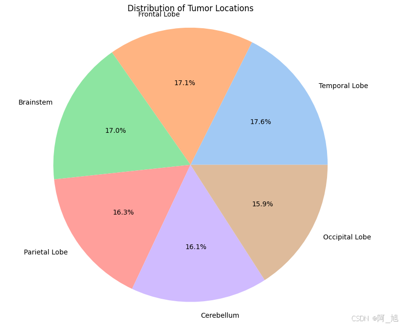
location_counts = data['Location'].value_counts()
plt.figure(figsize=(8, 8))
plt.pie(location_counts, labels=location_counts.index, autopct='%1.1f%%', colors=sns.color_palette('pastel'))
plt.title('Distribution of Tumor Locations')
plt.axis('equal')
plt.show()
2.数据预处理
2.1 数据特征编码与on-hot处理
#Data Preprocessing
from sklearn.model_selection import train_test_split
from sklearn.preprocessing import LabelEncoder,OneHotEncoder
import pandas as pd


data['Gender'] = LabelEncoder().fit_transform(data['Gender'])  # Encode Gender (0 for Female, 1 for Male)
data['Location'] = LabelEncoder().fit_transform(data['Location'])  # Encode Location
data['Grade'] = LabelEncoder().fit_transform(data['Grade'])

data['Tumor Type'] = LabelEncoder().fit_transform(data['Tumor Type'])  # Encode Tumor Type


columns = ['Gender','Location','Grade']
enc = OneHotEncoder()
# 将['Gender','Location','Grade']这3列进行独热编码
new_data = enc.fit_transform(data[columns]).toarray()
new_data.shape
(1000, 12)
data.head()
| Tumor Type | Location | Size (cm) | Grade | Patient Age | Gender | |
|---|---|---|---|---|---|---|
| 0 | 4 | 3 | 9.23 | 0 | 48 | 0 |
| 1 | 1 | 3 | 0.87 | 1 | 47 | 1 |
| 2 | 3 | 3 | 2.33 | 1 | 12 | 0 |
| 3 | 1 | 3 | 1.45 | 2 | 38 | 0 |
| 4 | 1 | 0 | 6.45 | 0 | 35 | 0 |
from sklearn.preprocessing import StandardScaler
# 1、实例化一个转换器类
transfer = StandardScaler()
# 2、调用fit_transform
data[['Size (cm)','Patient Age']] = transfer.fit_transform(data[['Size (cm)','Patient Age']])
old_data = data[['Tumor Type','Size (cm)','Patient Age']]
old_data.head()
one_hot_data = pd.DataFrame(new_data)
one_hot_data.head()
| 0 | 1 | 2 | 3 | 4 | 5 | 6 | 7 | 8 | 9 | 10 | 11 | |
|---|---|---|---|---|---|---|---|---|---|---|---|---|
| 0 | 1.0 | 0.0 | 0.0 | 0.0 | 0.0 | 1.0 | 0.0 | 0.0 | 1.0 | 0.0 | 0.0 | 0.0 |
| 1 | 0.0 | 1.0 | 0.0 | 0.0 | 0.0 | 1.0 | 0.0 | 0.0 | 0.0 | 1.0 | 0.0 | 0.0 |
| 2 | 1.0 | 0.0 | 0.0 | 0.0 | 0.0 | 1.0 | 0.0 | 0.0 | 0.0 | 1.0 | 0.0 | 0.0 |
| 3 | 1.0 | 0.0 | 0.0 | 0.0 | 0.0 | 1.0 | 0.0 | 0.0 | 0.0 | 0.0 | 1.0 | 0.0 |
| 4 | 1.0 | 0.0 | 1.0 | 0.0 | 0.0 | 0.0 | 0.0 | 0.0 | 1.0 | 0.0 | 0.0 | 0.0 |
final_data =pd.concat([old_data, one_hot_data], axis=1)
final_data.head()
| Tumor Type | Size (cm) | Patient Age | 0 | 1 | 2 | 3 | 4 | 5 | 6 | 7 | 8 | 9 | 10 | 11 | |
|---|---|---|---|---|---|---|---|---|---|---|---|---|---|---|---|
| 0 | 4 | 1.418484 | 0.179288 | 1.0 | 0.0 | 0.0 | 0.0 | 0.0 | 1.0 | 0.0 | 0.0 | 1.0 | 0.0 | 0.0 | 0.0 |
| 1 | 1 | -1.539861 | 0.139277 | 0.0 | 1.0 | 0.0 | 0.0 | 0.0 | 1.0 | 0.0 | 0.0 | 0.0 | 1.0 | 0.0 | 0.0 |
| 2 | 3 | -1.023212 | -1.261097 | 1.0 | 0.0 | 0.0 | 0.0 | 0.0 | 1.0 | 0.0 | 0.0 | 0.0 | 1.0 | 0.0 | 0.0 |
| 3 | 1 | -1.334617 | -0.220819 | 1.0 | 0.0 | 0.0 | 0.0 | 0.0 | 1.0 | 0.0 | 0.0 | 0.0 | 0.0 | 1.0 | 0.0 |
| 4 | 1 | 0.434728 | -0.340851 | 1.0 | 0.0 | 1.0 | 0.0 | 0.0 | 0.0 | 0.0 | 0.0 | 1.0 | 0.0 | 0.0 | 0.0 |
final_data.info()
<class 'pandas.core.frame.DataFrame'>
RangeIndex: 1000 entries, 0 to 999
Data columns (total 15 columns):
 #   Column       Non-Null Count  Dtype
---  ------       --------------  -----
 0   Tumor Type   1000 non-null   int64
 1   Size (cm)    1000 non-null   float64
 2   Patient Age  1000 non-null   float64
 3   0            1000 non-null   float64
 4   1            1000 non-null   float64
 5   2            1000 non-null   float64
 6   3            1000 non-null   float64
 7   4            1000 non-null   float64
 8   5            1000 non-null   float64
 9   6            1000 non-null   float64
 10  7            1000 non-null   float64
 11  8            1000 non-null   float64
 12  9            1000 non-null   float64
 13  10           1000 non-null   float64
 14  11           1000 non-null   float64
dtypes: float64(14), int64(1)
memory usage: 117.3 KB
3.模型训练与调优
3.1 数据划分
# Defining features and target
X = final_data.iloc[:,1:].values
y = final_data['Tumor Type'].values  # Example target variable

# Splitting data into training and testing sets
X_train, X_test, y_train, y_test = train_test_split(X, y, test_size=0.2, random_state=42)
X_train.shape
(800, 14)
3.2 模型训练调优
from sklearn.model_selection import train_test_split
from sklearn.svm import SVC
from sklearn.metrics import classification_report, accuracy_score, confusion_matrix
import matplotlib.pyplot as plt
from sklearn.model_selection import GridSearchCV

param_grid = {
    'C': [0.1, 1, 10, 100],
    'kernel': ['linear', 'poly', 'rbf', 'sigmoid'],
    'degree': [3, 5]  # 仅对多项式核有效
}
grid_search = GridSearchCV(SVC(random_state=42), param_grid, cv=5, n_jobs=-1)
grid_search.fit(X_train, y_train)
best_params = grid_search.best_params_
print("Best Parameters from Grid Search:")
print(best_params)
Best Parameters from Grid Search:
{'C': 0.1, 'degree': 3, 'kernel': 'linear'}
3.3 模型评估
best_model = grid_search.best_estimator_
y_pred = best_model.predict(X_test)
print("Best Model Classification Report:")
print(classification_report(y_test, y_pred))
# Print Confusion Matrix
print(confusion_matrix(y_test, y_pred))
好了,这篇文章就介绍到这里,如果对你有帮助,感谢点赞关注!