- 第三次作业
- 计算题
- 编程题
- 1 基于降维的机器学习
- 2 深度学习训练方法总结
第三次作业
计算题
- (15 分)对于给定矩阵 A A A(规模为 4×2),求 A A A 的 SVD(奇异值分解),即求 U U U, Σ Σ Σ, V T V^T VT, 使得 A = U Σ V T A = UΣV^T A=UΣVT。其中 U T U = I U^TU = I UTU=I, V T V = I V^TV = I VTV=I,给出求解过程。
A = [ 1 0 0 1 2 1 − 1 0 ] A= \begin{bmatrix} 1 & 0 \\ 0 &1 \\ 2 & 1 \\ -1 & 0 \end{bmatrix} A= 102−10110
【解】
首先计算
A
T
A
A^TA
ATA:
A
T
A
=
[
6
2
2
2
]
A^TA= \begin{bmatrix} 6&2\\ 2&2\\ \end{bmatrix}
ATA=[6222]
其特征值和单位特征向量分别为:
[
2
(
2
+
2
)
,
2
(
2
−
2
)
]
\begin{bmatrix} 2 (2 + \sqrt{2}), 2 (2 - \sqrt{2}) \end{bmatrix}
[2(2+2),2(2−2)]
V = [ 1 + 2 1 + ( 1 + 2 ) 2 1 − 2 1 + ( 1 − 2 ) 2 1 1 + ( 1 + 2 ) 2 1 1 + ( 1 − 2 ) 2 ] V = \begin{bmatrix} \frac{1 + \sqrt{2}}{\sqrt{1 + (1 + \sqrt{2})^2}} & \frac{1 - \sqrt{2}}{\sqrt{1 + (1 - \sqrt{2})^2}}\\ \frac{1}{\sqrt{1 + (1 + \sqrt{2})^2}} & \frac{1}{\sqrt{1 + (1 - \sqrt{2})^2}}\\ \end{bmatrix} V= 1+(1+2)21+21+(1+2)211+(1−2)21−21+(1−2)21
奇异值
σ
1
=
2
(
2
+
2
)
\sigma_1 = \sqrt{2 (2 + \sqrt{2})}
σ1=2(2+2),
σ
2
=
2
(
2
−
2
)
\sigma_2 = \sqrt{2 (2 - \sqrt{2})}
σ2=2(2−2),因此:
Σ
=
[
2
(
2
+
2
)
0
0
2
(
2
−
2
)
0
0
0
0
]
Σ = \begin{bmatrix} \sqrt{2 (2 + \sqrt{2})} & 0\\ 0 & \sqrt{2 (2 - \sqrt{2})}\\ 0 & 0\\ 0 & 0\\ \end{bmatrix}
Σ=
2(2+2)00002(2−2)00
记
U
=
(
u
1
,
u
2
,
u
3
,
u
4
)
U = (u_1,u_2,u_3,u_4)
U=(u1,u2,u3,u4),根据
A
V
=
U
Σ
AV=U\Sigma
AV=UΣ:
U
Σ
=
(
u
1
,
u
2
,
u
3
,
u
4
)
[
2
(
2
+
2
)
0
0
2
(
2
−
2
)
0
0
0
0
]
=
(
2
(
2
+
2
)
u
1
,
2
(
2
−
2
)
u
2
)
\begin{aligned} U\Sigma &= (u_1,u_2,u_3,u_4) \begin{bmatrix} \sqrt{2 (2 + \sqrt{2})} & 0\\ 0 & \sqrt{2 (2 - \sqrt{2})}\\ 0 & 0\\ 0 & 0\\ \end{bmatrix}\\ &=(\sqrt{2 (2 + \sqrt{2})}u_1,\sqrt{2 (2 - \sqrt{2})}u_2) \end{aligned}
UΣ=(u1,u2,u3,u4)
2(2+2)00002(2−2)00
=(2(2+2)u1,2(2−2)u2)
A V = [ 1 + 2 2 ( 2 + 2 ) 1 − 2 4 − 2 2 1 2 ( 2 + 2 ) 1 4 − 2 2 3 + 2 2 2 ( 2 + 2 ) 3 − 2 2 4 − 2 2 − 1 + 2 2 ( 2 + 2 ) − 1 − 2 2 ( 2 − 2 ) ] AV = \begin{bmatrix}\frac{1 + \sqrt{2}}{\sqrt{2(2+\sqrt{2})}} & \frac{1 - \sqrt{2}}{\sqrt{4-2\sqrt{2}}}\\\frac{1}{\sqrt{2(2+\sqrt{2})}} & \frac{1}{\sqrt{4-2\sqrt{2}}}\\\frac{3 + 2\sqrt{2}}{\sqrt{2(2+\sqrt{2})}} & \frac{3 - 2\sqrt{2}}{\sqrt{4-2\sqrt{2}}}\\-\frac{1 + \sqrt{2}}{\sqrt{2(2+\sqrt{2})}} & -\frac{1 - \sqrt{2}}{\sqrt{2(2-\sqrt{2})}}\\\end{bmatrix} AV= 2(2+2)1+22(2+2)12(2+2)3+22−2(2+2)1+24−221−24−2214−223−22−2(2−2)1−2
因此可得:
u
1
=
1
2
(
2
+
2
)
[
1
+
2
1
3
+
2
2
−
1
−
2
]
,
u
2
=
1
2
(
2
−
2
)
[
1
−
2
1
3
−
2
2
−
1
+
2
]
u_1=\frac{1}{2(2+\sqrt{2})} \begin{bmatrix} 1+\sqrt{2}\\ 1\\ 3+2\sqrt{2}\\ -1-\sqrt{2} \end{bmatrix}, u_2=\frac{1}{2(2-\sqrt{2})} \begin{bmatrix} 1-\sqrt{2}\\ 1\\ 3-2\sqrt{2}\\ -1+\sqrt{2} \end{bmatrix}
u1=2(2+2)1
1+213+22−1−2
,u2=2(2−2)1
1−213−22−1+2
扩展为标准正交基得:
U
=
[
1
+
2
2
(
2
+
2
)
1
−
2
2
(
2
−
2
)
1
2
−
1
2
1
2
(
2
+
2
)
1
2
(
2
−
2
)
0
−
1
2
3
+
2
2
2
(
2
+
2
)
3
−
2
2
(
2
−
2
)
0
1
2
−
1
−
2
2
(
2
+
2
)
2
−
1
2
(
2
−
2
)
1
2
1
2
]
U = \begin{bmatrix}\frac{1 + \sqrt{2}}{2(2+\sqrt{2})} & \frac{1 - \sqrt{2}}{2(2-\sqrt{2})} & \frac{1}{\sqrt{2}} & -\frac{1}{2}\\\frac{1}{2(2+\sqrt{2})} & \frac{1}{2(2-\sqrt{2})} & 0 & -\frac{1}{2}\\\frac{3 + 2\sqrt{2}}{2(2+\sqrt{2})} & \frac{3 - \sqrt{2}}{2(2-\sqrt{2})} & 0 & \frac{1}{2}\\\frac{-1 - \sqrt{2}}{2(2+\sqrt{2})} & \frac{\sqrt{2} - 1}{2(2-\sqrt{2})} & \frac{1}{\sqrt{2}} & \frac{1}{2}\\\end{bmatrix}
U=
2(2+2)1+22(2+2)12(2+2)3+222(2+2)−1−22(2−2)1−22(2−2)12(2−2)3−22(2−2)2−1210021−21−212121
最终,
A
=
U
Σ
V
T
=
[
1
+
2
2
(
2
+
2
)
1
−
2
2
(
2
−
2
)
1
2
−
1
2
1
2
(
2
+
2
)
1
2
(
2
−
2
)
0
−
1
2
3
+
2
2
2
(
2
+
2
)
3
−
2
2
(
2
−
2
)
0
1
2
−
1
−
2
2
(
2
+
2
)
2
−
1
2
(
2
−
2
)
1
2
1
2
]
[
2
(
2
+
2
)
0
0
2
(
2
−
2
)
0
0
0
0
]
[
1
+
2
1
+
(
1
+
2
)
2
1
1
+
(
1
+
2
)
2
1
−
2
1
+
(
1
−
2
)
2
1
1
+
(
1
−
2
)
2
]
A=U\Sigma V^T=\begin{bmatrix}\frac{1 + \sqrt{2}}{2(2+\sqrt{2})} & \frac{1 - \sqrt{2}}{2(2-\sqrt{2})} & \frac{1}{\sqrt{2}} & -\frac{1}{2}\\\frac{1}{2(2+\sqrt{2})} & \frac{1}{2(2-\sqrt{2})} & 0 & -\frac{1}{2}\\\frac{3 + 2\sqrt{2}}{2(2+\sqrt{2})} & \frac{3 - \sqrt{2}}{2(2-\sqrt{2})} & 0 & \frac{1}{2}\\\frac{-1 - \sqrt{2}}{2(2+\sqrt{2})} & \frac{\sqrt{2} - 1}{2(2-\sqrt{2})} & \frac{1}{\sqrt{2}} & \frac{1}{2}\\\end{bmatrix} \begin{bmatrix} \sqrt{2 (2 + \sqrt{2})} & 0\\ 0 & \sqrt{2 (2 - \sqrt{2})}\\ 0 & 0\\ 0 & 0\\ \end{bmatrix} \begin{bmatrix} \frac{1 + \sqrt{2}}{\sqrt{1 + (1 + \sqrt{2})^2}} & \frac{1}{\sqrt{1 + (1 + \sqrt{2})^2}}\\ \frac{1 - \sqrt{2}}{\sqrt{1 + (1 - \sqrt{2})^2}} & \frac{1}{\sqrt{1 + (1 - \sqrt{2})^2}}\\ \end{bmatrix}
A=UΣVT=
2(2+2)1+22(2+2)12(2+2)3+222(2+2)−1−22(2−2)1−22(2−2)12(2−2)3−22(2−2)2−1210021−21−212121
2(2+2)00002(2−2)00
1+(1+2)21+21+(1−2)21−21+(1+2)211+(1−2)21
- (15 分)现有如下数据(5 个样本,4 个维度 ( A , B , C , D ) (A,B,C,D) (A,B,C,D)),⽤ P C A PCA PCA 将数据降到 2 维, 给出求解过程。
| A | B | C | D |
|---|---|---|---|
| 1 | 5 | 3 | 1 |
| 4 | -4 | 6 | 6 |
| 1 | 4 | 3 | 2 |
| 4 | 4 | 2 | 2 |
| 5 | 5 | 2 | 4 |
【解】
X
=
[
1
4
1
4
5
5
−
4
4
4
5
3
6
3
2
2
1
6
2
2
4
]
X = \begin{bmatrix} 1 & 4 & 1 & 4 & 5\\ 5 & -4 & 4 & 4 & 5\\ 3 & 6 & 3 & 2 & 2\\ 1 & 6 & 2 & 2 & 4 \end{bmatrix}
X=
15314−466143244225524
零均值化后的
X
X
X:
[
−
2
1
−
2
1
2
2.2
−
6.8
1.2
1.2
2.2
−
0.2
2.8
−
0.2
−
1.2
−
1.2
−
2
3
−
1
−
1
1
]
\begin{bmatrix} -2 & 1 & -2 & 1 & 2 \\ 2.2 & -6.8 & 1.2 & 1.2 & 2.2\\ -0.2 & 2.8 & -0.2 & -1.2 & -1.2\\ -2 & 3 & -1 & -1 & 1 \end{bmatrix}
−22.2−0.2−21−6.82.83−21.2−0.2−111.2−1.2−122.2−1.21
协方差矩阵
C
=
1
5
X
X
T
C=\frac{1}{5}XX^T
C=51XXT:
[
2.8
−
1.6
0
2
−
1.6
11.76
−
4.76
−
5
0
−
4.76
2.16
1.8
2
−
5
1.8
3.2
]
\begin{bmatrix} 2.8 & -1.6 & 0 & 2 \\ -1.6 & 11.76 & -4.76 & -5 \\ 0 & -4.76 & 2.16 & 1.8 \\ 2 & -5 & 1.8 & 3.2 \end{bmatrix}
2.8−1.602−1.611.76−4.76−50−4.762.161.82−51.83.2
其特征值及对应的特征向量(按行排列)为:
[
16.27660036
3.30704892
0.30518298
0.03116774
]
\begin{bmatrix} 16.27660036 & 3.30704892 & 0.30518298 & 0.03116774 \end{bmatrix}
[16.276600363.307048920.305182980.03116774]
[ 0.1582177 − 0.84232941 0.33404265 0.3922548 − 0.84205227 − 0.21992632 0.30154762 − 0.3894219 − 0.37915865 0.40046886 0.25782506 0.79334081 0.34950516 0.28589904 0.85499168 − 0.25514134 ] \begin{bmatrix} 0.1582177 &-0.84232941 & 0.33404265 & 0.3922548 \\-0.84205227 &-0.21992632 & 0.30154762 & -0.3894219 \\-0.37915865 & 0.40046886 & 0.25782506 & 0.79334081\\ 0.34950516 & 0.28589904 & 0.85499168 & -0.25514134\\ \end{bmatrix} 0.1582177−0.84205227−0.379158650.34950516−0.84232941−0.219926320.400468860.285899040.334042650.301547620.257825060.854991680.3922548−0.38942190.79334081−0.25514134
取前两行,即得到降维矩阵
P
P
P:
P
=
[
0.1582177
−
0.84232941
0.33404265
0.3922548
−
0.84205227
−
0.21992632
0.30154762
−
0.3894219
]
P=\begin{bmatrix} 0.1582177 & -0.84232941 & 0.33404265 & 0.3922548\\-0.84205227 & -0.21992632 & 0.30154762 & -0.3894219 \end{bmatrix}
P=[0.1582177−0.84205227−0.84232941−0.219926320.334042650.301547620.3922548−0.3894219]
Y
=
P
X
Y=PX
Y=PX 即为降维到
k
k
k 维后的数据(行代表属性、列代表样本):
[
−
3.02087823
7.99814153
−
1.78629402
−
1.64568358
−
1.5452857
1.91880091
0.32951437
1.74930533
−
1.0783991
−
2.9192215
]
\begin{bmatrix} -3.02087823 & 7.99814153 & -1.78629402& -1.64568358 & -1.5452857\\ 1.91880091 & 0.32951437 & 1.74930533 & -1.0783991 &-2.9192215\end{bmatrix}
[−3.020878231.918800917.998141530.32951437−1.786294021.74930533−1.64568358−1.0783991−1.5452857−2.9192215]
-
(15 分)假设有六个样本在⼆维空间中:
正样本:(1,1),(2,1),(2,3)
负样本:(-1,-1),(0,-3),(-2,-4)
使⽤⽀持向量机求划分平⾯,给出⽀持向量模型及求解过程。
【解】
根据数据, y 1 = y 2 = y 3 = 1 , y 4 = y 5 = y 6 = − 1 y_1=y_2=y_3=1,y_4=y_5=y_6=-1 y1=y2=y3=1,y4=y5=y6=−1。
设
w
=
(
w
1
,
w
2
)
T
w = (w_1,w_2)^T
w=(w1,w2)T,则问题可以表示为以下约束最优化问题:
minimize
w
,
b
1
2
(
w
1
2
+
w
2
2
)
subject to
{
w
1
+
w
2
+
b
≥
1
2
w
1
+
w
2
+
b
≥
1
2
w
1
+
3
w
2
+
b
≥
1
−
(
−
w
1
−
w
2
+
b
)
≥
1
−
(
0
w
1
−
3
w
2
+
b
)
≥
1
−
(
−
2
w
1
−
4
w
2
+
b
)
≥
1
\begin{aligned} & \underset{w, b}{\text{minimize}} && \frac{1}{2}(w_1^2 + w_2^2) \\ & \text{subject to} && \begin{cases} w_1 + w_2 + b \geq 1 \\ 2w_1 + w_2 + b \geq 1 \\ 2w_1 + 3w_2 + b \geq 1 \\ -(-w_1 - w_2 + b) \geq 1 \\ -(0w_1 - 3w_2 + b) \geq 1 \\ -(-2w_1 - 4w_2 + b) \geq 1 \\ \end{cases} \end{aligned}
w,bminimizesubject to21(w12+w22)⎩
⎨
⎧w1+w2+b≥12w1+w2+b≥12w1+3w2+b≥1−(−w1−w2+b)≥1−(0w1−3w2+b)≥1−(−2w1−4w2+b)≥1
解得:
{
w
1
=
1
2
w
2
=
1
2
b
=
0
\begin{cases} w_1 = \frac{1}{2} \\ w_2 = \frac{1}{2} \\ b=0 \end{cases}
⎩
⎨
⎧w1=21w2=21b=0
则最大间隔分离超平面为:
1
2
x
(
1
)
+
1
2
x
(
2
)
=
0
\frac{1}{2}x^{(1)}+\frac{1}{2}x^{(2)}=0
21x(1)+21x(2)=0
其中
x
1
=
(
1
,
1
)
T
x_1=(1,1)^T
x1=(1,1)T,
x
2
=
(
−
1
,
−
1
)
T
x_2=(-1,-1)^T
x2=(−1,−1)T 为支持向量。
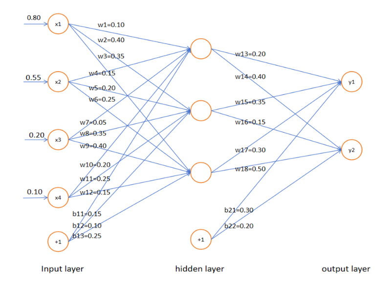
- (15 分)给定⼀个 4 ∗ 3 ∗ 2 4*3*2 4∗3∗2 的神经⽹络,权重矩阵为:
W 1 = [ 0.10 0.40 0.35 0.15 0.20 0.25 0.05 0.35 0.40 0.20 0.25 0.15 ] W_1= \begin{bmatrix} 0.10 & 0.40 & 0.35 \\ 0.15 & 0.20 & 0.25 \\ 0.05 & 0.35 & 0.40 \\ 0.20 & 0.25 & 0.15 \end{bmatrix} W1= 0.100.150.050.200.400.200.350.250.350.250.400.15
b 1 = [ 0.15 , 0.10 , 0.25 ] b_1=\begin{bmatrix}0.15 , 0.10 , 0.25 \end{bmatrix} b1=[0.15,0.10,0.25]
W 2 = [ 0.20 0.40 0.35 0.15 0.30 0.50 ] W_2= \begin{bmatrix} 0.20 & 0.40 \\ 0.35 & 0.15 \\ 0.30 & 0.50 \end{bmatrix} W2= 0.200.350.300.400.150.50
b 2 = [ 0.30 , 0.20 ] b_2 = \begin{bmatrix} 0.30, 0.20 \end{bmatrix} b2=[0.30,0.20]
激活函数为 sigmoid 函数。给定⼀个训练样本 x = [ 0.80 , 0.55 , 0.20 , 0.10 ] x=[0.80,0.55,0.20,0.10] x=[0.80,0.55,0.20,0.10] 和 y = [ 1 , 0 ] y=[1,0] y=[1,0],假设学习率为 0.01,损失函数为⼆元交叉熵损失,计算 w 10 , w 13 w_{10},w_{13} w10,w13 参数的⼀次更新结果。
【解】
(1)前向传播
a. 输入层到隐层
根据权重矩阵
W
1
W_1
W1 和偏置
b
1
b_1
b1 ,隐层的输入为:
a
1
=
W
1
T
x
1
+
b
1
=
[
0.10
0.15
0.05
0.20
0.40
0.20
0.35
0.25
0.35
0.25
0.40
0.15
]
[
0.80
0.55
0.20
0.10
]
+
[
0.15
0.10
0.25
]
=
[
0.3425
0.625
0.7625
]
a_1 = W_1^Tx_1+b_1=\begin{bmatrix} 0.10 & 0.15 & 0.05 & 0.20 \\ 0.40 & 0.20 & 0.35 & 0.25 \\ 0.35 & 0.25 & 0.40 & 0.15 \end{bmatrix}\begin{bmatrix}0.80 \\ 0.55 \\ 0.20 \\ 0.10 \end{bmatrix} + \begin{bmatrix}0.15 \\ 0.10 \\ 0.25 \end{bmatrix} = \begin{bmatrix}0.3425 \\ 0.625 \\ 0.7625 \end{bmatrix}
a1=W1Tx1+b1=
0.100.400.350.150.200.250.050.350.400.200.250.15
0.800.550.200.10
+
0.150.100.25
=
0.34250.6250.7625
在隐层经过 sigmoid 函数
σ
(
a
)
=
1
1
+
e
−
a
\sigma(a)=\frac{1}{1+e^{-a}}
σ(a)=1+e−a1 激活后:
h
1
=
σ
(
a
1
)
=
[
σ
(
0.3425
)
σ
(
0.625
)
σ
(
0.7625
)
]
≈
[
0.5848
0.6514
0.6819
]
h_1=\sigma(a_1)=\begin{bmatrix} \sigma(0.3425) \\ \sigma(0.625) \\ \sigma(0.7625) \end{bmatrix} \approx \begin{bmatrix} 0.5848 \\ 0.6514 \\ 0.6819 \end{bmatrix}
h1=σ(a1)=
σ(0.3425)σ(0.625)σ(0.7625)
≈
0.58480.65140.6819
b. 隐藏层到输出层
同理,输出层的输入为:
a
2
=
W
2
T
h
1
+
b
2
=
[
0.20
0.35
0.30
0.40
0.15
0.50
]
[
0.5848
0.6514
0.6819
]
+
[
0.30
0.20
]
=
[
0.8495
0.8726
]
a_2 = W_2^Th_1+b_2=\begin{bmatrix} 0.20 & 0.35 & 0.30 \\ 0.40 & 0.15 & 0.50 \end{bmatrix}\begin{bmatrix}0.5848 \\ 0.6514 \\ 0.6819 \end{bmatrix} + \begin{bmatrix}0.30 \\ 0.20 \end{bmatrix} = \begin{bmatrix} 0.8495 \\ 0.8726 \end{bmatrix}
a2=W2Th1+b2=[0.200.400.350.150.300.50]
0.58480.65140.6819
+[0.300.20]=[0.84950.8726]
输出层经过 sigmoid 激活函数后:
h
2
=
σ
(
a
2
)
=
[
σ
(
0.8495
)
σ
(
0.8726
)
]
≈
[
0.7005
0.7053
]
h_2=\sigma(a_2)=\begin{bmatrix} \sigma(0.8495) \\ \sigma(0.8726) \end{bmatrix} \approx \begin{bmatrix} 0.7005 \\ 0.7053 \end{bmatrix}
h2=σ(a2)=[σ(0.8495)σ(0.8726)]≈[0.70050.7053]
(2)计算损失
使用二元交叉熵损失,
L
(
y
,
h
2
)
=
−
1
N
∑
i
=
1
N
[
y
i
⋅
l
o
g
(
h
2
i
)
+
(
1
−
y
i
)
⋅
l
o
g
(
1
−
h
2
i
)
]
=
−
1
2
[
y
1
⋅
l
o
g
(
h
21
)
+
(
1
−
y
1
)
⋅
l
o
g
(
1
−
h
21
)
+
y
2
⋅
l
o
g
(
h
22
)
+
(
1
−
y
2
)
⋅
l
o
g
(
1
−
h
22
)
]
=
−
1
2
[
(
1
⋅
l
o
g
(
0.7005
)
+
(
1
−
1
)
⋅
l
o
g
(
1
−
0.7005
)
+
0
⋅
l
o
g
(
0.7053
)
+
(
1
−
0
)
⋅
l
o
g
(
1
−
0.7053
)
)
]
≈
0.7889
\begin{aligned} L(y,h_2) &=−\frac{1}{N}\sum_{i=1}^N[y_i⋅log( h_{2i})+(1−y_i)⋅log(1− h_{2i})] \\ &= −\frac{1}{2}[y_1 \cdot log( h_{21})+(1−y_1)\cdot log(1− h_{21})+y_2\cdot log( h_{22})+(1−y_2)\cdot log(1− h_{22})] \\ &= −\frac{1}{2}[(1\cdot log(0.7005)+(1−1) \cdot log(1−0.7005)+0\cdot log(0.7053)+(1−0) \cdot log(1−0.7053))] \\ &\approx 0.7889 \end{aligned}
L(y,h2)=−N1i=1∑N[yi⋅log(h2i)+(1−yi)⋅log(1−h2i)]=−21[y1⋅log(h21)+(1−y1)⋅log(1−h21)+y2⋅log(h22)+(1−y2)⋅log(1−h22)]=−21[(1⋅log(0.7005)+(1−1)⋅log(1−0.7005)+0⋅log(0.7053)+(1−0)⋅log(1−0.7053))]≈0.7889
其中,
y
i
y_i
yi 是第
i
i
i 个样本的真实值,
h
2
i
h_{2i}
h2i 是模型对第
i
i
i 个样本的预测值。
(3)反向传播
对
w
13
w_{13}
w13,
∂
L
∂
w
13
=
∂
L
∂
h
21
⋅
∂
h
21
∂
a
21
⋅
∂
a
21
∂
w
13
\frac{\partial L}{\partial w_{13}} = \frac{\partial L}{\partial h_{21}} \cdot \frac{\partial h_{21}}{\partial a_{21}} \cdot \frac{\partial a_{21}}{\partial w_{13}}
∂w13∂L=∂h21∂L⋅∂a21∂h21⋅∂w13∂a21
对于
y
1
=
1
y_1=1
y1=1,
∂
L
∂
h
21
=
−
(
y
1
h
21
−
1
−
y
1
1
−
h
21
)
=
−
1
h
21
≈
−
1.4276
\frac{\partial L}{\partial h_{21}}=-(\frac{y_1}{ h_{21}}-\frac{1-y_1}{1- h_{21}})=-\frac{1}{ h_{21}}\approx -1.4276
∂h21∂L=−(h21y1−1−h211−y1)=−h211≈−1.4276
由于
h
21
=
σ
(
a
21
)
=
1
1
+
e
−
a
21
h_{21} = \sigma(a_{21})=\frac{1}{1+e^{-a_{21}}}
h21=σ(a21)=1+e−a211,
∂
h
21
∂
a
21
=
h
21
(
1
−
h
21
)
=
0.7005
×
0.2995
≈
0.2098
\frac{\partial h_{21}}{\partial a_{21}}= h_{21}(1- h_{21})=0.7005 \times 0.2995 \approx 0.2098
∂a21∂h21=h21(1−h21)=0.7005×0.2995≈0.2098
又
a
2
=
(
w
13
w
15
w
17
)
T
⋅
h
1
+
b
2
a_{2}= \begin{pmatrix} w_{13} \\ w_{15} \\ w_{17} \end{pmatrix}^T \cdot h_1 + b_{2}
a2=
w13w15w17
T⋅h1+b2
因此,
∂
a
21
∂
w
13
=
h
11
=
0.5848
\frac{\partial a_{21}}{\partial w_{13}} = h_{11}=0.5848
∂w13∂a21=h11=0.5848
更新
w
13
w_{13}
w13 的值为:
w
13
=
w
13
−
η
⋅
∂
L
∂
w
13
=
0.2
−
0.01
×
(
−
1.4276
)
×
0.2098
×
0.5848
≈
0.2018
w_{13} = w_{13}-\eta \cdot \frac{\partial L}{\partial w_{13}} =0.2-0.01 \times (-1.4276)\times 0.2098 \times 0.5848 \approx 0.2018
w13=w13−η⋅∂w13∂L=0.2−0.01×(−1.4276)×0.2098×0.5848≈0.2018
同理可得,
w
14
≈
0.3959
w_{14}\approx 0.3959
w14≈0.3959。
对
w
10
w_{10}
w10,
∂
L
∂
w
10
=
∂
L
∂
h
11
⋅
∂
h
11
∂
a
11
⋅
∂
a
11
∂
w
10
=
∂
L
∂
h
11
⋅
[
h
11
⋅
(
1
−
h
11
)
]
⋅
x
4
=
∂
L
∂
h
11
⋅
0.2428
⋅
0.1
\frac{\partial L}{\partial w_{10}} = \frac{\partial L}{\partial h_{11}} \cdot \frac{\partial h_{11}}{\partial a_{11}} \cdot \frac{\partial a_{11}}{\partial w_{10}} = \frac{\partial L}{\partial h_{11}} \cdot [h_{11} \cdot (1-h_{11})]\cdot x_4 = \frac{\partial L}{\partial h_{11}} \cdot 0.2428 \cdot 0.1
∂w10∂L=∂h11∂L⋅∂a11∂h11⋅∂w10∂a11=∂h11∂L⋅[h11⋅(1−h11)]⋅x4=∂h11∂L⋅0.2428⋅0.1
其中,
h
11
h_{11}
h11 会接受
a
21
a_{21}
a21 和
a
22
a_{22}
a22 两个地方传来的误差,
∂
L
∂
h
11
=
∂
L
∂
a
21
⋅
∂
a
21
∂
h
11
+
∂
L
∂
a
22
⋅
∂
a
22
∂
h
11
=
−
1
a
21
⋅
w
13
+
[
(
−
1
a
22
)
⋅
w
14
]
≈
−
0.8494
\frac{\partial L}{\partial h_{11}} = \frac{\partial L}{\partial a_{21}} \cdot \frac{\partial a_{21}}{\partial h_{11}} + \frac{\partial L}{\partial a_{22}} \cdot \frac{\partial a_{22}}{\partial h_{11}} = -\frac{1}{a_{21}}\cdot w_{13} + [(-\frac{1}{a_{22}})\cdot w_{14}] \approx - 0.8494
∂h11∂L=∂a21∂L⋅∂h11∂a21+∂a22∂L⋅∂h11∂a22=−a211⋅w13+[(−a221)⋅w14]≈−0.8494
更新
w
10
w_{10}
w10 的值为:
w
10
=
w
10
−
η
⋅
∂
L
∂
w
10
=
0.1999
w_{10} = w_{10}-\eta \cdot \frac{\partial L}{\partial w_{10}} = 0.1999
w10=w10−η⋅∂w10∂L=0.1999
编程题
1 基于降维的机器学习
数据集:kddcup99_train.csv, kddcup99_test.csv
数据描述:https://www.kdd.org/kdd-cup/view/kdd-cup-1999/Data,⽬的是通过42维的数 据判断某⼀个数据包是否为 attack。(注意,数据中有多种类型的 attack,我们将他们统⼀ 认为是attack,不做具体区分,只区分normal和attack,可以预处理的时候把所有的attack 都统⼀ re-label,具体 attack 列表可参考 https://kdd.org/cupfiles/KDDCupData/1999/training_attack_types)。
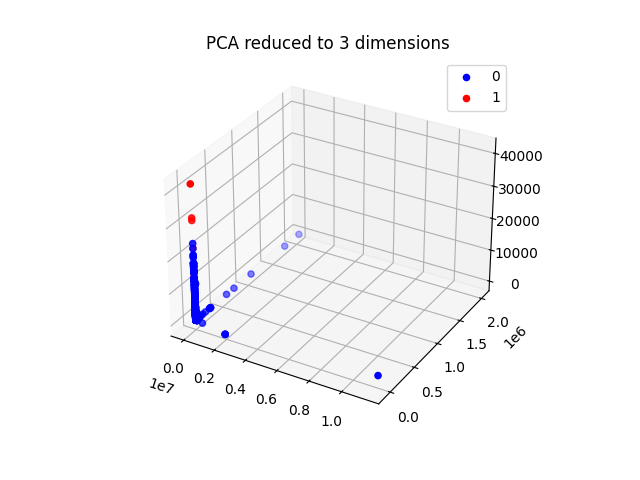
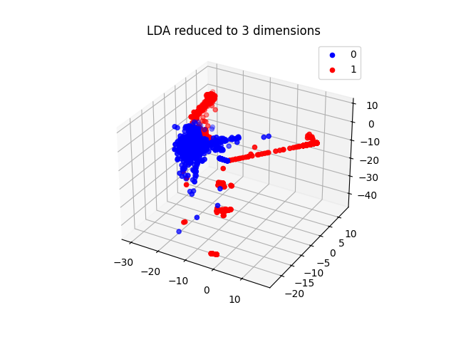
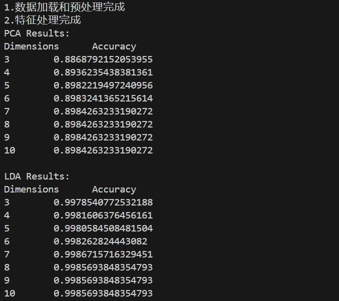
任务描述:选择 SVM,结合降维⽅法 PCALDA,实现数据降维+分类。
要求输出:不同⽅法降低到不同维度对判别结果的影响(提升还是下降),Plot 出两种降维 ⽅法降到 3 维之后的结果(Normal 和 Attack 的 sample ⽤不同颜⾊)
import pandas as pd
import numpy as np
from sklearn.preprocessing import LabelEncoder, StandardScaler, OneHotEncoder
from sklearn.compose import ColumnTransformer
from sklearn.decomposition import PCA
from sklearn.discriminant_analysis import LinearDiscriminantAnalysis as LDA
from sklearn.svm import SVC
from sklearn.metrics import accuracy_score
import matplotlib.pyplot as plt
from mpl_toolkits.mplot3d import Axes3D

# 创建列名列表, 数据集有 42 列(包括 41 个特征列和 1 个目标列)
column_names = [
    'duration', 'protocol_type', 'service', 'flag', 'src_bytes',
    'dst_bytes', 'land', 'wrong_fragment', 'urgent', 'hot',
    'num_failed_logins', 'logged_in', 'num_compromised', 'root_shell',
    'su_attempted', 'num_root', 'num_file_creations', 'num_shells',
    'num_access_files', 'num_outbound_cmds', 'is_host_login',
    'is_guest_login', 'count', 'srv_count', 'serror_rate',
    'srv_serror_rate', 'rerror_rate', 'srv_rerror_rate', 'same_srv_rate',
    'diff_srv_rate', 'srv_diff_host_rate', 'dst_host_count',
    'dst_host_srv_count', 'dst_host_same_srv_rate', 'dst_host_diff_srv_rate',
    'dst_host_same_src_port_rate', 'dst_host_srv_diff_host_rate',
    'dst_host_serror_rate', 'dst_host_srv_serror_rate', 'dst_host_rerror_rate',
    'dst_host_srv_rerror_rate', 'label'
]

# 加载数据, 跳过错误行
train = pd.read_csv('kddcup99_train.csv', names=column_names, on_bad_lines='skip')
test = pd.read_csv('kddcup99_test.csv', names=column_names, on_bad_lines='skip')

# 将训练集和测试集各缩小一百倍
train = train.sample(frac=0.01)
test = test.sample(frac=0.01)

print("1.数据加载和预处理完成")

# 对文本列进行编码
categorical_columns = ['protocol_type', 'service', 'flag']
for column in categorical_columns:
    combined_data = pd.concat([train[column], test[column]], axis=0)
    le = LabelEncoder()
    le.fit(combined_data)
    train[column] = le.transform(train[column])
    test[column] = le.transform(test[column])

X_train = train.drop(columns=['label'])
y_train = train['label']
y_train_relabel = y_train.apply(lambda x: 1 if x != 'normal.' else 0)
X_test = test.drop(columns=['label'])
y_test = test['label']
y_test_relabel = y_test.apply(lambda x: 1 if x != 'normal.' else 0)

print("2.特征处理完成")

# 定义降维函数
def reduce_dimension(reduction_method, X_train, y_train, X_test, n_components):
    if reduction_method == 'PCA':
        reducer = PCA(n_components=n_components)
    elif reduction_method == 'LDA':
        reducer = LDA(n_components=n_components)

    X_train_reduced = reducer.fit_transform(X_train, y_train)
    X_test_reduced = reducer.transform(X_test)

    return X_train_reduced, X_test_reduced

# 定义分类函数
def classify(X_train, y_train, X_test, y_test):
    clf = SVC()
    clf.fit(X_train, y_train)
    y_pred = clf.predict(X_test)

    accuracy = accuracy_score(y_test, y_pred)
    return accuracy, y_pred

# 降维和分类
results = {'PCA': [], 'LDA': []}

for dim in range(3,11):
    X_train_pca, X_test_pca = reduce_dimension('PCA', X_train, y_train, X_test, dim)
    accuracy_pca, _ = classify(X_train_pca, y_train_relabel, X_test_pca, y_test_relabel)
    results['PCA'].append((dim, accuracy_pca))

    X_train_lda, X_test_lda = reduce_dimension('LDA', X_train, y_train, X_test, dim)
    accuracy_lda, _ = classify(X_train_lda, y_train_relabel, X_test_lda, y_test_relabel)
    results['LDA'].append((dim, accuracy_lda))

print("PCA Results:")
print(f"Dimensions\tAccuracy")
for dim, acc in results['PCA']:
    print(dim,"\t", acc)

print("\nLDA Results:")
print(f"Dimensions\tAccuracy")
for dim, acc in results['LDA']:
    print(dim,"\t", acc)

# 可视化降到3维的结果
X_train_pca_3d, _ = reduce_dimension('PCA', X_train, y_train, X_test, 3)
X_train_lda_3d, _ = reduce_dimension('LDA', X_train, y_train, X_test, 3)

def plot_3d(X, y, title):
    fig = plt.figure()
    ax = fig.add_subplot(111, projection='3d')
    ax.set_title(title)

    colors = {0: 'b', 1: 'r'}  # 0: normal, 1: attack
    for label in np.unique(y):
        ax.scatter(X[y == label, 0], X[y == label, 1], X[y == label, 2], c=colors[label], label=label, s=20)

    ax.legend()
    plt.show()

plot_3d(X_train_pca_3d, y_train_relabel, "PCA reduced to 3 dimensions")
plot_3d(X_train_lda_3d, y_train_relabel, "LDA reduced to 3 dimensions")
2 深度学习训练方法总结
数据集:kddcup99_Train.csv, kddcup99_Test.csv ,数据的每一行有 42 列,根据前 41 列的值去预测第42列是否为 attack。
任务描述:实现⼀个简单的神经网络模型判别数据包是否为attack,网络层数不小于5层,,例如 41->36->24->12->6->1。
要求至少 2 种激活函数,至少 2 种 parameter initialization 方法,至少 2 种训练方法(SGD,SGD+Momentom,Adam)。
训练模型并判断训练结果。
要求输出:
1)模型描述,层数,每⼀层参数,激活函数选择,loss 函数设置等;
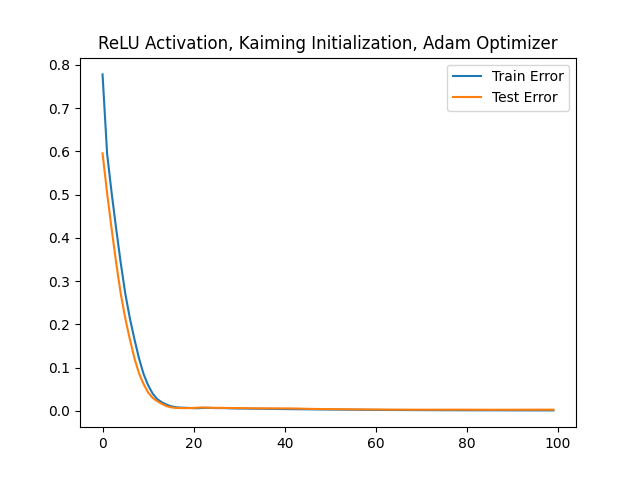
2)针对不同方法组合(至少 2 个组合),plot 出随着 epoch 增长 training error 和 test error 的变化情况。
import torch
import torch.nn as nn
import torch.optim as optim
import pandas as pd
import matplotlib.pyplot as plt
from sklearn.preprocessing import LabelEncoder
from sklearn.preprocessing import StandardScaler
from colorama import Fore, Style

# Load data
train_data = pd.read_csv('kddcup99_train.csv', header= None, on_bad_lines='skip')
test_data = pd.read_csv('kddcup99_test.csv', header= None, on_bad_lines='skip')

# 将训练集和测试集各缩小一百倍
train_data = train_data.sample(frac=0.01)
test_data = test_data.sample(frac=0.01)

# 对文本列进行编码
categorical_columns = train_data.columns[1:4].tolist()
for column in categorical_columns:
    combined_data = pd.concat([train_data[column], test_data[column]], axis=0)
    le = LabelEncoder()
    le.fit(combined_data)
    train_data[column] = le.transform(train_data[column])
    test_data[column] = le.transform(test_data[column])


X_train = train_data.iloc[:, :-1]
y_train = train_data.iloc[:, -1]
y_train_relabel = y_train.apply(lambda x: 1 if x != 'normal.' else 0)
X_test = test_data.iloc[:, :-1]
y_test = test_data.iloc[:, -1]
y_test_relabel = y_test.apply(lambda x: 1 if x != 'normal.' else 0)

#  X_train  X_test normalization
sc = StandardScaler()
X_train = sc.fit_transform(X_train)
X_test = sc.transform(X_test)

# Convert to tensors
X_train = torch.tensor(X_train, dtype=torch.float)
y_train_relabel = torch.tensor(y_train_relabel.values, dtype=torch.float)
X_test = torch.tensor(X_test, dtype=torch.float)
y_test_relabel = torch.tensor(y_test_relabel.values, dtype=torch.float)

# Define the network
class Net(nn.Module):
    def __init__(self, activation):
        super(Net, self).__init__()
        self.fc1 = nn.Linear(41, 36)
        self.fc2 = nn.Linear(36, 24)
        self.fc3 = nn.Linear(24, 12)
        self.fc4 = nn.Linear(12, 6)
        self.fc5 = nn.Linear(6, 1)

        if activation == 'relu':
            self.activation = nn.ReLU()
        elif activation == 'sigmoid':
            self.activation = nn.Sigmoid()

    def forward(self, x):
        x = self.activation(self.fc1(x))
        x = self.activation(self.fc2(x))
        x = self.activation(self.fc3(x))
        x = self.activation(self.fc4(x))
        x = torch.sigmoid(self.fc5(x))  # final activation is sigmoid for binary classification
        return x

# Training function
def train(net, X_train, y_train, X_test, y_test, optimizer, criterion, epochs=100):
    train_errors = []
    test_errors = []
    for epoch in range(epochs):
        optimizer.zero_grad()
        output = net(X_train).squeeze()  # squeeze the output to remove the extra dimension
        train_loss = criterion(output, y_train)
        train_loss.backward()
        optimizer.step()

        # Record errors
        train_error = train_loss.item()
        test_output = net(X_test).squeeze()  # squeeze the output here too
        test_loss = criterion(test_output, y_test)
        test_error = test_loss.item()
        train_errors.append(train_error)
        test_errors.append(test_error)

        if epoch % 10 == 0:
            print(Fore.GREEN + 'epoch: [{:3d}/{}], '.format(epoch, epochs) + Fore.BLUE + 'train step: {}, '.format(epoch) + Fore.RED + 'train_loss: {:.5f}, '.format(train_error) + Fore.YELLOW + 'test_loss: {:.5f}'.format(test_error))

    print(Style.RESET_ALL)  # Reset the color to default
    return train_errors, test_errors

# Initialize network with ReLU activation, Xavier initialization, and SGD optimizer
net = Net('sigmoid')
nn.init.xavier_uniform_(net.fc1.weight)
nn.init.xavier_uniform_(net.fc2.weight)
nn.init.xavier_uniform_(net.fc3.weight)
nn.init.xavier_uniform_(net.fc4.weight)
nn.init.xavier_uniform_(net.fc5.weight)
optimizer = optim.SGD(net.parameters(), lr=0.01)
criterion = nn.BCELoss()

# Train and plot errors
train_errors, test_errors = train(net, X_train, y_train_relabel, X_test, y_test_relabel, optimizer, criterion)

print("Model structure: ", net, "\n\n")

for name, param in net.named_parameters():
    print(f"Layer: {name} | Size: {param.size()} | Values : {param[:2]} \n")

plt.title('Sigmoid Activation, Xavier Initialization, SGD Optimizer')
plt.plot(train_errors, label='Train Error')
plt.plot(test_errors, label='Test Error')
plt.legend()
plt.show()

# Initialize network with Sigmoid activation, Kaiming initialization, and Adam optimizer
net = Net('relu')
nn.init.kaiming_uniform_(net.fc1.weight)
nn.init.kaiming_uniform_(net.fc2.weight)
nn.init.kaiming_uniform_(net.fc3.weight)
nn.init.kaiming_uniform_(net.fc4.weight)
nn.init.kaiming_uniform_(net.fc5.weight)
optimizer = optim.Adam(net.parameters(), lr=0.01)


# Train and plot errors
train_errors, test_errors = train(net, X_train, y_train_relabel, X_test, y_test_relabel, optimizer, criterion)

print("Model structure: ", net, "\n\n")

for name, param in net.named_parameters():
    print(f"Layer: {name} | Size: {param.size()} | Values : {param[:2]} \n")

plt.title('ReLU Activation, Kaiming Initialization, Adam Optimizer')
plt.plot(train_errors, label='Train Error')
plt.plot(test_errors, label='Test Error')
plt.legend()
plt.show()
输出:
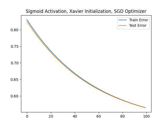
epoch: [  0/100], train step: 0, train_loss: 0.83076, test_loss: 0.82476
epoch: [ 10/100], train step: 10, train_loss: 0.77907, test_loss: 0.77409
epoch: [ 20/100], train step: 20, train_loss: 0.73555, test_loss: 0.73146
epoch: [ 30/100], train step: 30, train_loss: 0.69899, test_loss: 0.69566
epoch: [ 40/100], train step: 40, train_loss: 0.66831, test_loss: 0.66563
epoch: [ 50/100], train step: 50, train_loss: 0.64258, test_loss: 0.64046
epoch: [ 60/100], train step: 60, train_loss: 0.62099, test_loss: 0.61933
epoch: [ 70/100], train step: 70, train_loss: 0.60285, test_loss: 0.60160
epoch: [ 80/100], train step: 80, train_loss: 0.58759, test_loss: 0.58668
epoch: [ 90/100], train step: 90, train_loss: 0.57472, test_loss: 0.57411

Model structure:  Net(
  (fc1): Linear(in_features=41, out_features=36, bias=True)
  (fc2): Linear(in_features=36, out_features=24, bias=True)
  (fc3): Linear(in_features=24, out_features=12, bias=True)
  (fc4): Linear(in_features=12, out_features=6, bias=True)
  (fc5): Linear(in_features=6, out_features=1, bias=True)
  (activation): Sigmoid()
)


Layer: fc1.weight | Size: torch.Size([36, 41]) | Values : tensor([[-0.1204,  0.1695, -0.0945, -0.1015, -0.0338, -0.0430, -0.2108, -0.0487,
          0.2591,  0.0264, -0.2337,  0.1409, -0.2239,  0.1533,  0.1117, -0.1207,
          0.1573,  0.2463, -0.1667,  0.2229,  0.2368,  0.0499, -0.0194,  0.1738,
          0.0057,  0.2606, -0.1390, -0.2654, -0.1701,  0.0092, -0.0232, -0.2021,
         -0.1327, -0.0356,  0.2128,  0.0905, -0.2579,  0.0700, -0.2245,  0.1827,
          0.0351],
        [-0.0199, -0.0828,  0.1850,  0.2518,  0.1650, -0.0836, -0.0384,  0.0219,
          0.0745,  0.0179, -0.1767, -0.2702, -0.1961,  0.2151,  0.1896, -0.0962,
         -0.2253,  0.2759, -0.0934, -0.0413, -0.1034,  0.2449,  0.2524, -0.0120,
          0.1045,  0.0078,  0.1084, -0.0260, -0.2767, -0.1596, -0.1660,  0.1970,
          0.2388,  0.0917, -0.1074,  0.1396,  0.2334, -0.2057, -0.0928,  0.0844,
          0.2253]], grad_fn=<SliceBackward0>)

Layer: fc1.bias | Size: torch.Size([36]) | Values : tensor([-0.0125, -0.0647], grad_fn=<SliceBackward0>)

Layer: fc2.weight | Size: torch.Size([24, 36]) | Values : tensor([[ 0.1901,  0.3076,  0.2780, -0.1221,  0.0865, -0.1958, -0.1591,  0.2710,
         -0.0584,  0.0713,  0.1986,  0.0998,  0.0596,  0.1909,  0.1504,  0.1529,
         -0.0607,  0.0267, -0.2466, -0.0994,  0.3090,  0.0109,  0.1064, -0.2247,
          0.0065, -0.2745, -0.2972,  0.1079, -0.2792, -0.2592, -0.0671,  0.1319,
          0.1867, -0.2757, -0.0122,  0.3061],
        [-0.2875,  0.0513, -0.2721,  0.1229,  0.1980, -0.2237,  0.0273,  0.0966,
         -0.1452, -0.1988, -0.0604, -0.0344, -0.2188,  0.1212, -0.1144, -0.2195,
          0.0199,  0.1941,  0.0436, -0.0758,  0.2529,  0.0526,  0.1667,  0.0497,
          0.1492, -0.0510,  0.1750,  0.1225, -0.1053,  0.1485,  0.2058,  0.2799,
         -0.0877, -0.0516, -0.1451, -0.0730]], grad_fn=<SliceBackward0>)

Layer: fc2.bias | Size: torch.Size([24]) | Values : tensor([ 0.0214, -0.1065], grad_fn=<SliceBackward0>)

Layer: fc3.weight | Size: torch.Size([12, 24]) | Values : tensor([[ 0.0663, -0.1093,  0.1332,  0.0015,  0.0130, -0.0853, -0.1504,  0.4016,
          0.1938, -0.3305,  0.0805, -0.4046,  0.1531,  0.2350,  0.2465, -0.3746,
          0.1722, -0.0767,  0.2982,  0.3774,  0.3722, -0.0244,  0.3968,  0.0536],
        [-0.3444,  0.3722,  0.1660,  0.1776, -0.3715, -0.3797, -0.3049, -0.3762,
          0.3245,  0.4026, -0.0206,  0.0601,  0.3001, -0.2587,  0.3230,  0.1495,
          0.1577,  0.1810, -0.1501,  0.3237, -0.0502,  0.2333, -0.2059, -0.1671]],
       grad_fn=<SliceBackward0>)

Layer: fc3.bias | Size: torch.Size([12]) | Values : tensor([ 0.0377, -0.0293], grad_fn=<SliceBackward0>)

Layer: fc4.weight | Size: torch.Size([6, 12]) | Values : tensor([[ 0.4014,  0.2608, -0.0577,  0.4244,  0.1046,  0.4315,  0.3025, -0.1401,
         -0.3695,  0.3276,  0.4545, -0.5888],
        [ 0.5549, -0.1166, -0.2757, -0.0290,  0.2277, -0.4197, -0.3324, -0.4567,
         -0.2027, -0.2449,  0.3914,  0.4241]], grad_fn=<SliceBackward0>)

Layer: fc4.bias | Size: torch.Size([6]) | Values : tensor([0.0023, 0.1753], grad_fn=<SliceBackward0>)

Layer: fc5.weight | Size: torch.Size([1, 6]) | Values : tensor([[-0.5094,  0.8143,  0.8610,  0.4556, -0.2517, -0.0298]],
       grad_fn=<SliceBackward0>)

Layer: fc5.bias | Size: torch.Size([1]) | Values : tensor([-0.0002], grad_fn=<SliceBackward0>)

epoch: [  0/100], train step: 0, train_loss: 0.77802, test_loss: 0.59542
epoch: [ 10/100], train step: 10, train_loss: 0.05965, test_loss: 0.04284
epoch: [ 20/100], train step: 20, train_loss: 0.00630, test_loss: 0.00698
epoch: [ 30/100], train step: 30, train_loss: 0.00557, test_loss: 0.00664
epoch: [ 40/100], train step: 40, train_loss: 0.00429, test_loss: 0.00585
epoch: [ 50/100], train step: 50, train_loss: 0.00323, test_loss: 0.00419
epoch: [ 60/100], train step: 60, train_loss: 0.00241, test_loss: 0.00331
epoch: [ 70/100], train step: 70, train_loss: 0.00185, test_loss: 0.00287
epoch: [ 80/100], train step: 80, train_loss: 0.00154, test_loss: 0.00289
epoch: [ 90/100], train step: 90, train_loss: 0.00137, test_loss: 0.00280

Model structure:  Net(
  (fc1): Linear(in_features=41, out_features=36, bias=True)
  (fc2): Linear(in_features=36, out_features=24, bias=True)
  (fc3): Linear(in_features=24, out_features=12, bias=True)
  (fc4): Linear(in_features=12, out_features=6, bias=True)
  (fc5): Linear(in_features=6, out_features=1, bias=True)
  (activation): ReLU()
)


Layer: fc1.weight | Size: torch.Size([36, 41]) | Values : tensor([[-0.2223,  0.2652,  0.2620, -0.1737,  0.3073, -0.0071, -0.1844, -0.0910,
         -0.3330, -0.3644,  0.1672,  0.1811, -0.1323,  0.1138,  0.2474,  0.1190,
          0.0716,  0.2176, -0.2005, -0.2051,  0.2049, -0.2390,  0.1245, -0.3129,
          0.2679,  0.2085, -0.2465,  0.3374, -0.3995, -0.1678,  0.0991,  0.2571,
         -0.2904, -0.3289,  0.1882, -0.2960, -0.2482,  0.2063,  0.4326,  0.0245,
          0.3398],
        [-0.0233,  0.4540, -0.2002, -0.1890,  0.3571, -0.0085,  0.1579,  0.3280,
          0.0949,  0.1917,  0.2366,  0.2644,  0.1930, -0.4022,  0.2962, -0.1272,
         -0.1952, -0.1286, -0.2101,  0.2916,  0.2925,  0.4614, -0.2036, -0.1995,
          0.0267, -0.1885,  0.1940,  0.2943, -0.0280, -0.0546,  0.3826,  0.0526,
          0.1689,  0.5428, -0.2704, -0.1747, -0.0180, -0.2829,  0.2023,  0.1309,
          0.0611]], grad_fn=<SliceBackward0>)

Layer: fc1.bias | Size: torch.Size([36]) | Values : tensor([-0.0362,  0.0334], grad_fn=<SliceBackward0>)

Layer: fc2.weight | Size: torch.Size([24, 36]) | Values : tensor([[ 0.2063,  0.1689,  0.1686, -0.0299, -0.1831,  0.0941,  0.2320, -0.3211,
          0.1923,  0.0230,  0.4319, -0.1799,  0.1243, -0.3534, -0.1607,  0.0783,
          0.1387, -0.3061,  0.3025, -0.2749,  0.1129,  0.1131,  0.0264,  0.2124,
          0.0571,  0.1330,  0.2580,  0.1441, -0.2470,  0.1353, -0.2976,  0.1211,
         -0.4715, -0.3144,  0.3093,  0.0863],
        [-0.1541,  0.3662, -0.0299,  0.0588,  0.4050,  0.1201,  0.0695, -0.1545,
          0.3148, -0.0187, -0.0606, -0.2249,  0.2707, -0.3788,  0.3024,  0.1695,
          0.1224,  0.0702, -0.3575,  0.3632, -0.4167,  0.0654, -0.4184, -0.0808,
          0.1539,  0.3601,  0.2400, -0.1469,  0.0635,  0.4880, -0.2289,  0.2739,
         -0.3789,  0.0521,  0.1561,  0.1686]], grad_fn=<SliceBackward0>)

Layer: fc2.bias | Size: torch.Size([24]) | Values : tensor([-0.1722, -0.1973], grad_fn=<SliceBackward0>)

Layer: fc3.weight | Size: torch.Size([12, 24]) | Values : tensor([[-0.3522,  0.3949, -0.4170, -0.0109, -0.0345, -0.0263,  0.1290,  0.2439,
         -0.4594, -0.0283, -0.3729,  0.4788,  0.2042,  0.3306, -0.3264, -0.2471,
          0.3756, -0.2152, -0.1101,  0.2048, -0.1268, -0.3149, -0.2185,  0.1856],
        [-0.0387,  0.3687, -0.3605,  0.1807, -0.1386,  0.1414,  0.4445,  0.5877,
         -0.1079,  0.2080, -0.3797,  0.3645,  0.1634, -0.2281,  0.4158, -0.5624,
          0.2715,  0.4161,  0.1966, -0.3475, -0.1538,  0.4041,  0.0800,  0.5462]],
       grad_fn=<SliceBackward0>)

Layer: fc3.bias | Size: torch.Size([12]) | Values : tensor([-0.1063,  0.0016], grad_fn=<SliceBackward0>)

Layer: fc4.weight | Size: torch.Size([6, 12]) | Values : tensor([[ 0.3684,  0.3588,  0.4967,  0.4015, -0.6398, -0.2540,  0.2881, -0.4240,
         -0.2107,  0.1753, -0.0842,  0.5281],
        [ 0.0090, -0.4973,  0.6199, -0.4902,  0.1952,  0.6437, -0.5067,  0.5859,
          0.8092,  0.8759,  0.0526, -0.3403]], grad_fn=<SliceBackward0>)

Layer: fc4.bias | Size: torch.Size([6]) | Values : tensor([-0.2995,  0.0266], grad_fn=<SliceBackward0>)

Layer: fc5.weight | Size: torch.Size([1, 6]) | Values : tensor([[-0.0259, -0.4790,  0.7276,  0.2180,  0.6982, -0.7128]],
       grad_fn=<SliceBackward0>)

Layer: fc5.bias | Size: torch.Size([1]) | Values : tensor([0.0468], grad_fn=<SliceBackward0>)