讲解关于slam一系列文章汇总链接:史上最全slam从零开始,针对于本栏目讲解(02)Cartographer源码无死角解析-链接如下:
(02)Cartographer源码无死角解析- (00)目录_最新无死角讲解:https://blog.csdn.net/weixin_43013761/article/details/127350885
文末正下方中心提供了本人
联系方式,
点击本人照片即可显示
W
X
→
官方认证
{\color{blue}{文末正下方中心}提供了本人 \color{red} 联系方式,\color{blue}点击本人照片即可显示WX→官方认证}
文末正下方中心提供了本人联系方式,点击本人照片即可显示WX→官方认证
一、前言
在上一篇博客中,对ceres扫描匹配的平移与旋转优化部分进行了详细的讲解,知道关于ceres的使用核心在于禅茶的构建。不过,留下了两个疑问暂时比较迷糊:
疑问 1 \color{red}疑问1 疑问1 与 疑问 2 \color{red}疑问2 疑问2 整合:CeresScanMatcher2D::Match()函数中,为什么平移残差优化的目标是 target_translation(由推断器或者暴力匹配获得),为什么旋转的残差目标值设置为 ceres_pose_estimate[2]。暂且记住这两个疑问,看下接下来的分析中是否能够找到答案。
下面要分析的是 src/cartographer/cartographer/mapping/internal/2d/scan_matching/ceres_scan_matcher_2d.cc 文件中的 CeresScanMatcher2D::Match() 函数的如下部分:
  // 地图部分的残差
  CHECK_GT(options_.occupied_space_weight(), 0.);
  switch (grid.GetGridType()) {
    case GridType::PROBABILITY_GRID:
      problem.AddResidualBlock(
          CreateOccupiedSpaceCostFunction2D(
              options_.occupied_space_weight() /
                  std::sqrt(static_cast<double>(point_cloud.size())),
              point_cloud, grid),
          nullptr /* loss function */, ceres_pose_estimate);
      break;
    case GridType::TSDF:
      problem.AddResidualBlock(
          CreateTSDFMatchCostFunction2D(
              options_.occupied_space_weight() /
                  std::sqrt(static_cast<double>(point_cloud.size())),
              point_cloud, static_cast<const TSDF2D&>(grid)),
          nullptr /* loss function */, ceres_pose_estimate);
      break;
  }
由于目前使用的是概率栅格地图,所以只对上述的 case GridType::PROBABILITY_GRID 情况进行讲解,即其核心函数为 CreateOccupiedSpaceCostFunction2D(),该函数主要作用是构建一个 ceres::CostFunction 对象指针返回作为 problem.AddResidualBlock() 函数的第一个实参。这里与平移旋转的优化一样 loss function 设置为 nullptr 表示不使用损失函数,CreateOccupiedSpaceCostFunction2D() 函数最后接收的参数 ceres_pose_estimate 表示待优化位姿的初始值。
那么下面就来详细分析一下吧。
二、CreateOccupiedSpaceCostFunction2D()
首先这里粘贴一下该函数的代码:
// 工厂函数, 返回地图的CostFunction
ceres::CostFunction* CreateOccupiedSpaceCostFunction2D(
    const double scaling_factor, const sensor::PointCloud& point_cloud,
    const Grid2D& grid) {
  return new ceres::AutoDiffCostFunction<OccupiedSpaceCostFunction2D,
                                         ceres::DYNAMIC /* residuals */,
                                         3 /* pose variables */>(
      new OccupiedSpaceCostFunction2D(scaling_factor, point_cloud, grid),
      point_cloud.size()); // 比固定残差维度的 多了一个参数
}
首先其是一个工厂函数,第一个形参表示 scaling_factor 表示残差结果的所缩放因子;第二个形参 point_cloud 表示需要进行扫描匹配的点云数据,也是待优化的点云数据;第三个形参 grid 存储了栅格地图的相关数据与信息,后续会使用到。
ceres::AutoDiffCostFunction 类模板根据根据上述的三个形参构建一个:
ceres::AutoDiffCostFunction<OccupiedSpaceCostFunction2D,
                                         ceres::DYNAMIC /* residuals */,
                                         3 /* pose variables */>
类对象,第一个模板参数OccupiedSpaceCostFunction2D是一个可调用类型(可以是仿函数,或者可调用对象);第二个非类型模板参数 ceres::DYNAMIC=-1 与上一篇博客讲解的有些不一样,这里是一个动态值,也就是说残差结果项是动态的,需要在程序执行过程中才能确定(主要与点云数量相关);第三个非类型模板参数3表示位姿,也就是前面参数 ceres_pose_estimate(位姿初始值) 的维度,简单的说,就是待优化变量的维度。
创建上述类模板的实例,需要传递两个参数,第一个参数为可调用类型 OccupiedSpaceCostFunction2D 的实例对象,第二个参数为 point_cloud.size(),只有在 ceres::DYNAMIC=-1,即残差项为动态的情况下,才需要传入该参数,其目的就是指定残差项的维度。
三、GridArrayAdapter
从上面的分析中可以明显知道,class OccupiedSpaceCostFunction2D 这个类是栅格地图优化的核心,不过在对齐进行讲解之前,先来看 class GridArrayAdapter 这个类,该类同样实现于 occupied_space_cost_function_2d.cc 文件中,且被包含在类 OccupiedSpaceCostFunction2D 之中。
GridArrayAdapter 类型实例主要用于创建类模板 ceres::BiCubicInterpolator 的实例对象,ceres::BiCubicInterpolator 的作用是进行双线性插值。其对需要进行插值的实例对象有一定要求,在本人人在 /usr/include/ceres/cubic_interpolation.h 中关于 ceres::BiCubicInterpolator 的介绍,可以找到如下内容:
// Given as input an infinite two dimensional grid like object, which
// provides the following interface:
//
//   struct Grid {
//     enum { DATA_DIMENSION = 1 };
//     void GetValue(int row, int col, double* f) const;
//   };
//
// Where, GetValue gives us the value of a function f (possibly vector
// valued) for any pairs of integers (row, col), and the enum
// DATA_DIMENSION indicates the dimensionality of the function being
// interpolated. For example if you are interpolating a color image
// with three channels (Red, Green & Blue), then DATA_DIMENSION = 3.
大概的意思:如果使用 ceres::BiCubicInterpolator 进行双线性插值,需要实现一个结构体(或者类) Grid,用该类创建的实例对象作为 ceres::BiCubicInterpolator 构造函数的实参。关于 Grid 这个结构体需要实现两个接口:①enum { DATA_DIMENSION = 1 }用于指定数据的维度;②GetValue函数,该函数返回指定行列(int row, int col)位置的value值。
源码中的 Grid 结构体,就是 class GridArrayAdapte,是严格按照上述要求进行实现的。并且还额外实现了 NumRows() 与 NumCols() 函数,在GetValue() 函数重被调用,需要注意的是,其对 map上下左右各增加 kPadding,也就是对 map 进行了填充。相关代码注释如下:
private:
  static constexpr int kPadding = INT_MAX / 4;

  // 自定义网格
  class GridArrayAdapter {
   public:
    // 枚举 DATA_DIMENSION 表示被插值的向量或者函数的维度
    enum { DATA_DIMENSION = 1 };

    explicit GridArrayAdapter(const Grid2D& grid) : grid_(grid) {}

    // 获取栅格free值
    void GetValue(const int row, const int column, double* const value) const {
      // 处于地图外部时, 赋予最大free值
      if (row < kPadding || column < kPadding || row >= NumRows() - kPadding ||
          column >= NumCols() - kPadding) {
        *value = kMaxCorrespondenceCost;
      }
      // 根据索引获取free值
      else {
        *value = static_cast<double>(grid_.GetCorrespondenceCost(
            Eigen::Array2i(column - kPadding, row - kPadding)));
      }
    }

    // map上下左右各增加 kPadding
    int NumRows() const {
      return grid_.limits().cell_limits().num_y_cells + 2 * kPadding;
    }

    int NumCols() const {
      return grid_.limits().cell_limits().num_x_cells + 2 * kPadding;
    }

   private:
    const Grid2D& grid_;
  };
实现了 GridArrayAdapter 之后,后续就能够通过如下代码进行双线性插值了:
    const GridArrayAdapter adapter(grid_);
    ceres::BiCubicInterpolator<GridArrayAdapter> interpolator(adapter);
关于双线性插值的知识,这里就不进行讲解了,不是很明白的朋友可以查阅一些其他的资料。总的来说,没有插值之前,我们只能通过整数索引 (int row, const int column) 获得栅格值,但是通过插值之后,就可以通过小数索引获得栅格值了。
四、OccupiedSpaceCostFunction2D
首先这里讲解一下优化的原理:①待优化的参数为机器人位姿,即 CeresScanMatcher2D::Match() 函数中ceres_pose_estimate变量,其使用二维的方式表示机器人位姿,即位置(x,y),角度(angle)。②优化之后的最终结果是希望所有点云数据都能够打在障碍物上,即点云数据对应的栅格值(没有被占用概率)越小越好,也就说,点云对应的栅格值越小,则其被占用的机率越大。
1.源码注释
先简单过一下源码的注释,然后再对其重难点进行分袖
class OccupiedSpaceCostFunction2D {
 public:
  OccupiedSpaceCostFunction2D(const double scaling_factor,
                              const sensor::PointCloud& point_cloud,
                              const Grid2D& grid)
      : scaling_factor_(scaling_factor),//残差项的缩放因子
        point_cloud_(point_cloud),//当前扫描匹配的点云数据
        grid_(grid) {}//存储有地图栅格信息

  template <typename T>
  bool operator()(const T* const pose, T* residual) const {
    Eigen::Matrix<T, 2, 1> translation(pose[0], pose[1]);//二维位置
    Eigen::Rotation2D<T> rotation(pose[2]);//二维角度(姿态)
    //把角度使用2x2矩阵形式表示
    Eigen::Matrix<T, 2, 2> rotation_matrix = rotation.toRotationMatrix();

    /*姿态与位姿都添加到3x3的矩阵中,构成类似: r1 r2  tx 的矩阵形式
                                           r3 r4  ty
                                           0. 0.  1.          */
    Eigen::Matrix<T, 3, 3> transform;
    transform << rotation_matrix, translation, T(0.), T(0.), T(1.);

    //对地图进行双线性插值,ceres的基本使用形式
    const GridArrayAdapter adapter(grid_);
    ceres::BiCubicInterpolator<GridArrayAdapter> interpolator(adapter);

    const MapLimits& limits = grid_.limits(); //获取地图边界信息

    //循环遍历进行扫描匹配的点云数据
    for (size_t i = 0; i < point_cloud_.size(); ++i) {
      // Note that this is a 2D point. The third component is a scaling factor.
      // 由于点云数据经过重力校正,所以只取x,y坐标
      const Eigen::Matrix<T, 3, 1> point((T(point_cloud_[i].position.x())),
                                         (T(point_cloud_[i].position.y())),
                                         T(1.));
      // 根据预测位姿对单个点进行坐标变换
      // 这里把point看成一个向量, 该向量的原点未local系, 向量的长度
      // 该向量的长度点云数据的模,所以还需要对齐进行变换,等价于把
      // 该向量的原点移动至Robot系原点,但是点云数据的数字是相对于loacl系的
      const Eigen::Matrix<T, 3, 1> world = transform * point;

      // 获取三次插值之后的栅格free值, Evaluate函数内部调用了GetValue函数
      interpolator.Evaluate(
          (limits.max().x() - world[0]) / limits.resolution() - 0.5 +
              static_cast<double>(kPadding),
          (limits.max().y() - world[1]) / limits.resolution() - 0.5 +
              static_cast<double>(kPadding),
          &residual[i]);
      // free值越小, 表示占用的概率越大
      // 希望residual[i]为0,即希望每个点云都打在障碍物上,也就是等价
      // 点云对应栅格值越小越好
      residual[i] = scaling_factor_ * residual[i];
    }
    return true;
  }

 private:
  static constexpr int kPadding = INT_MAX / 4;

  OccupiedSpaceCostFunction2D(const OccupiedSpaceCostFunction2D&) = delete;
  OccupiedSpaceCostFunction2D& operator=(const OccupiedSpaceCostFunction2D&) =
      delete;

  const double scaling_factor_;
  const sensor::PointCloud& point_cloud_;
  const Grid2D& grid_;
};
2.重难点分析
其上的大部分代码都是比较容易理解的,但是对于如下部分代码或许存在一定疑问:
const Eigen::Matrix<T, 3, 1> world = transform * point;
下面是本人绘画的图示,①黄色圆点表示点云数据;②紫色五边形表示机器人所在位置及朝向;③黑色矩形表示障碍物;

从上图可以看到,点云数据虽然位于local坐标系下,但是很明显是不能计算残差的。需要把点云数据变换到如下位置才能进行残差计算:

上述源码就是为了实现上述功能,需要注意的是,源码中的 point 与 world 都是基于local 系的。从上图很容易看出,point 基于local系进行平移与旋转即可变换成 world,其平移与旋转的量就是机器人在local系下的位姿。使用数学公式表示则如下所示:
p
o
i
n
t
t
r
a
c
k
i
n
g
l
o
c
a
l
=
R
o
b
o
t
t
r
a
c
k
i
n
g
l
o
c
a
l
∗
p
o
i
n
t
l
o
c
a
l
(01)
\color{Green} \tag{01} point^{local}_{tracking}=\mathbf {Robot}^{local}_{tracking}*point^{local}
pointtrackinglocal=Robottrackinglocal∗pointlocal(01)
p
o
i
n
t
t
r
a
c
k
i
n
g
l
o
c
a
l
point^{local}_{tracking}
pointtrackinglocal 表是的含义就是对 local 系下的向量,起点为 tracking(机器人),终点为点云数值。
五、结语
通过上一篇博客与该篇博客的讲解,可以知道扫描匹配核心函数 CeresScanMatcher2D::Match() 主要是对初始位姿 ceres_pose_estimate 进行优化,优化主要包含如下三个步骤:
①首先根据点云数据,结合栅格地图进行位姿优化,尽量让所有的点云数据都打在障碍物上。
②以推断器推断出来位置target_translation作为优化目标,计算x,y的残差。
③以ceres_pose_estimate[2]作为角度优化目标,该残差也只计算了角度这一项。
这里再重述一下上一篇博客遗留的疑问→ 疑问 1 \color{red}疑问1 疑问1 与 疑问 2 \color{red}疑问2 疑问2 整合:CeresScanMatcher2D::Match()函数中,为什么平移残差优化的目标是 target_translation(由推断器或者暴力匹配获得),为什么旋转的残差目标值设置为 ceres_pose_estimate[2]。
CeresScanMatcher2D::Match() 的三个残差块都可以通过配置文件中的 occupied_space_weight、translation_weight、rotation_weight 对残差结果进行缩放。
总的来说,Cartographer源码是比较信任推断器的的,所以②使用target_translation作为优化目标,起到一个约束作用,避免优化过程中跑偏了。①的优化可能会导致角度发生得到优化,即ceres_pose_estimate[2]发生变化,但是源码中似乎认为推断器推断出来的姿态是十分准确的,并不想对齐进行优化,所以用初值作为优化目标,尽量保证其值不变。