目录
💥1 概述
📚2 运行结果
🎉3 参考文献
👨💻4 Matlab代码
💥1 概述
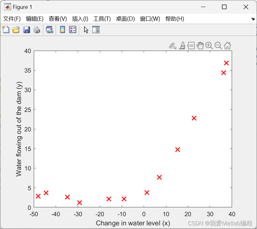
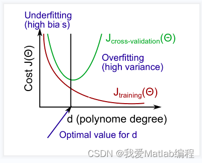
本文使用水库水位的变化来实现正则化线性回归,以预测大坝流出的水量。后续本文将对调试学习算法进行一些诊断,并检查偏差与方差的影响。
第 1 部分:正则化线性回归
我们将实现正则化线性回归,以利用水库水位的变化来预测从大坝流出的水量。
第 1.1 部分:加载和可视化数据
我们将首先可视化包含有关水位变化 x 和从大坝流出的水量 y 的历史记录的数据集。
此数据集分为三个部分:
- 模型将学习的训练集:X, y
- 用于确定正则化参数的交叉验证集:Xval、yval
- 用于评估性能的测试集。这些是你的模型在训练过程中没有看到的“看不见的”例子:Xtest,ytest。
📚2 运行结果


🎉3 参考文献
[1]刘建伟,崔立鹏,刘泽宇,罗雄麟.正则化稀疏模型[J].计算机学报,2015,38(07):1307-1325.
👨💻4 Matlab代码
主函数部分代码:
%% Initialization
clear ; close all; clc
%% =========== Part 1: Loading and Visualizing Data =============
% We start the exercise by first loading and visualizing the dataset.
% The following code will load the dataset into your environment and plot
% the data.
%
% Load Training Data
fprintf('Loading and Visualizing Data ...\n')
% Load from ex5data1:
% You will have X, y, Xval, yval, Xtest, ytest in your environment
load ('ex5data1.mat');
% m = Number of examples
m = size(X, 1);
% Plot training data
plot(X, y, 'rx', 'MarkerSize', 10, 'LineWidth', 1.5);
xlabel('Change in water level (x)');
ylabel('Water flowing out of the dam (y)');
fprintf('Program paused. Press enter to continue.\n');
pause;
%% =========== Part 2: Regularized Linear Regression Cost =============
% You should now implement the cost function for regularized linear
% regression.
%
theta = [1 ; 1];
J = linearRegCostFunction([ones(m, 1) X], y, theta, 1);
fprintf(['Cost at theta = [1 ; 1]: %f '...
'\n(this value should be about 303.993192)\n'], J);
fprintf('Program paused. Press enter to continue.\n');
pause;
%% =========== Part 3: Regularized Linear Regression Gradient =============
% You should now implement the gradient for regularized linear
% regression.
%
theta = [1 ; 1];
[J, grad] = linearRegCostFunction([ones(m, 1) X], y, theta, 1);
fprintf(['Gradient at theta = [1 ; 1]: [%f; %f] '...
'\n(this value should be about [-15.303016; 598.250744])\n'], ...
grad(1), grad(2));
fprintf('Program paused. Press enter to continue.\n');
pause;
%% =========== Part 4: Train Linear Regression =============
% Once you have implemented the cost and gradient correctly, the
% trainLinearReg function will use your cost function to train
% regularized linear regression.
%
% Write Up Note: The data is non-linear, so this will not give a great
% fit.
%
% Train linear regression with lambda = 0
lambda = 0;
[theta] = trainLinearReg([ones(m, 1) X], y, lambda);
% Plot fit over the data
plot(X, y, 'rx', 'MarkerSize', 10, 'LineWidth', 1.5);
xlabel('Change in water level (x)');
ylabel('Water flowing out of the dam (y)');
hold on;
plot(X, [ones(m, 1) X]*theta, '--', 'LineWidth', 2)
hold off;
fprintf('Program paused. Press enter to continue.\n');
pause;
%% =========== Part 5: Learning Curve for Linear Regression =============
% Next, you should implement the learningCurve function.
%
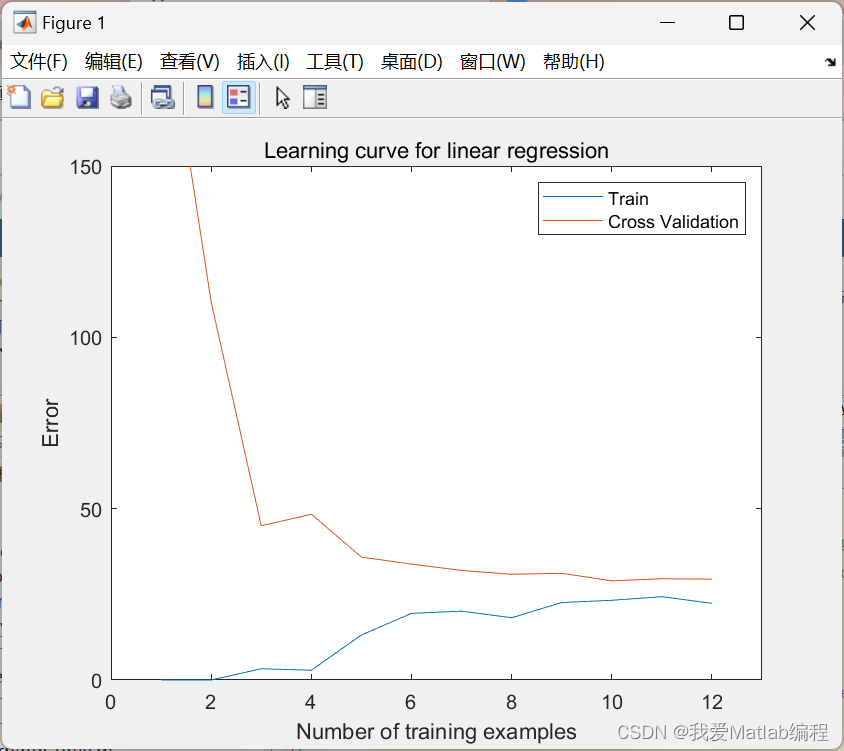
% Write Up Note: Since the model is underfitting the data, we expect to
% see a graph with "high bias" -- Figure 3 in ex5.pdf
%
lambda = 0;
[error_train, error_val] = ...
learningCurve([ones(m, 1) X], y, ...
[ones(size(Xval, 1), 1) Xval], yval, ...
lambda);
plot(1:m, error_train, 1:m, error_val);
title('Learning curve for linear regression')
legend('Train', 'Cross Validation')
xlabel('Number of training examples')
ylabel('Error')
axis([0 13 0 150])
fprintf('# Training Examples\tTrain Error\tCross Validation Error\n');
for i = 1:m
fprintf(' \t%d\t\t%f\t%f\n', i, error_train(i), error_val(i));
end