本文主要包含以下内容:
- 推导神经网络的误差反向传播过程
- 使用numpy编写简单的神经网络,并使用iris数据集和california_housing数据集分别进行分类和回归任务,最终将训练过程可视化。
1. BP算法的推导过程
1.1 导入
前向传播和反向传播的总体过程。
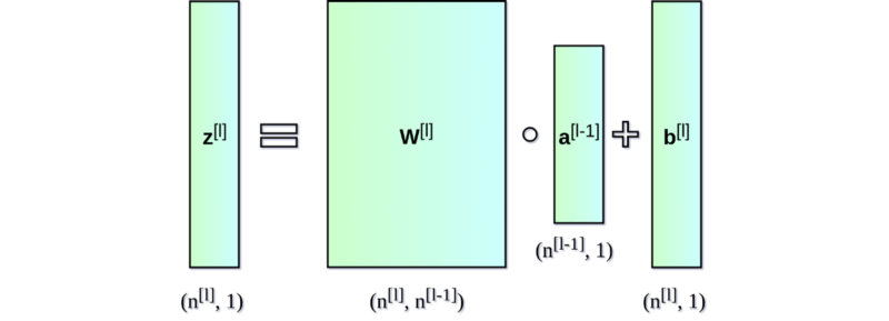
神经网络的直接输出记为
Z
[
l
]
Z^{[l]}
Z[l],表示激活前的输出,激活后的输出记为
A
A
A。
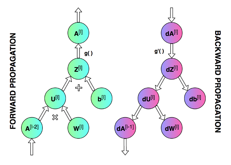
第一个图像是神经网络的前向传递和反向传播的过程,第二个图像用于解释中间的变量关系,第三个图像是前向和后向过程的计算图,方便进行推导,但是第三个图左下角的 A [ l − 2 ] A^{[l-2]} A[l−2]有错误,应该是 A [ l − 1 ] A^{[l-1]} A[l−1]。
1.2 符号表
为了方便进行推导,有必要对各个符号进行介绍
符号表
| 记号 | 含义 |
|---|---|
| n l n_l nl | 第 l l l层神经元个数 |
| f l ( ⋅ ) f_l(\cdot) fl(⋅) | 第 l l l层神经元的激活函数 |
| W l ∈ R n l − 1 × n l \mathbf{W}^l\in\R^{n_{l-1}\times n_{l}} Wl∈Rnl−1×nl | 第 l − 1 l-1 l−1层到第 l l l层的权重矩阵 |
| b l ∈ R n l \mathbf{b}^l \in \R^{n_l} bl∈Rnl | 第 l − 1 l-1 l−1层到第 l l l层的偏置 |
| Z l ∈ R n l \mathbf{Z}^l \in \R^{n_l} Zl∈Rnl | 第 l l l层的净输出,没有经过激活的输出 |
| A l ∈ R n l \mathbf{A}^l \in \R^{n_l} Al∈Rnl | 第 l l l层经过激活函数的输出, A 0 = X A^0=X A0=X |
深层的神经网络都是由一个一个单层网络堆叠起来的,于是我们可以写出神经网络最基本的结构,然后进行堆叠得到深层的神经网络。
于是,我们可以开始编写代码,通过一个类Layer来描述单个神经网络层
class Layer:
    def __init__(self, input_dim, output_dim):
        # 初始化参数
        self.W = np.random.randn(input_dim, output_dim) * 0.01
        self.b = np.zeros((1, output_dim))

    def forward(self, X):
        # 前向计算
        self.Z = np.dot(X, self.W) + self.b
        self.A = self.activation(self.Z)
        return self.A

    def backward(self, dA, A_prev, activation_derivative):
        # 反向传播
        # 计算公式推导见下方
        m = A_prev.shape[0]
        self.dZ = dA * activation_derivative(self.Z)
        self.dW = np.dot(A_prev.T, self.dZ) / m
        self.db = np.sum(self.dZ, axis=0, keepdims=True) / m
        dA_prev = np.dot(self.dZ, self.W.T)
        return dA_prev

    def update_parameters(self, learning_rate):
        # 参数更新
        self.W -= learning_rate * self.dW
        self.b -= learning_rate * self.db


# 带有ReLU激活函数的Layer
class ReLULayer(Layer):
    def activation(self, Z):
        return np.maximum(0, Z)

    def activation_derivative(self, Z):
        return (Z > 0).astype(float)

# 带有Softmax激活函数(主要用于分类)的Layer
class SoftmaxLayer(Layer):
    def activation(self, Z):
        exp_z = np.exp(Z - np.max(Z, axis=1, keepdims=True))
        return exp_z / np.sum(exp_z, axis=1, keepdims=True)

    def activation_derivative(self, Z):
        # Softmax derivative is more complex, not directly used in this form.
        return np.ones_like(Z)
1.3 推导过程
权重更新的核心在于计算得到self.dW和self.db,同时,为了将梯度信息不断回传,需要backward函数返回梯度信息dA_prev。
需要用到的公式
Z
l
=
W
l
A
l
−
1
+
b
l
A
l
=
f
(
Z
l
)
d
Z
d
W
=
(
A
l
−
1
)
T
d
Z
d
b
=
1
Z^l = W^l A^{l-1} +b^l \\A^l = f(Z^l)\\\frac{dZ}{dW} = (A^{l-1})^T \\\frac{dZ}{db} = 1
Zl=WlAl−1+blAl=f(Zl)dWdZ=(Al−1)TdbdZ=1
解释:
从上方计算图右侧的反向传播过程可以看到,来自于上一层的梯度信息dA经过dZ之后直接传递到db,也经过dU之后传递到dW,于是我们可以得到dW和db的梯度计算公式如下:
d
W
=
d
A
⋅
d
A
d
Z
⋅
d
Z
d
W
=
d
A
⋅
f
′
(
d
Z
)
⋅
A
p
r
e
v
T
\begin{align}dW &= dA \cdot \frac{dA}{dZ} \cdot \frac{dZ}{dW}\\ &= dA \cdot f'(dZ) \cdot A_{prev}^T \\ \end{align}
dW=dA⋅dZdA⋅dWdZ=dA⋅f′(dZ)⋅AprevT
其中,
f
(
⋅
)
f(\cdot)
f(⋅)是激活函数,
f
′
(
⋅
)
f'(\cdot)
f′(⋅)是激活函数的导数,
A
p
r
e
v
T
A_{prev}^T
AprevT是当前层上一层激活输出的转置。
同理,可以得到
d
b
=
d
A
⋅
d
A
d
Z
⋅
d
Z
d
b
=
d
A
⋅
f
′
(
d
Z
)
\begin{align}db &= dA \cdot \frac{dA}{dZ} \cdot \frac{dZ}{db}\\ &= dA \cdot f'(dZ) \\ \end{align}
db=dA⋅dZdA⋅dbdZ=dA⋅f′(dZ)
需要仅需往前传递的梯度信息:
d
A
p
r
e
v
=
d
A
⋅
d
A
d
Z
⋅
d
Z
A
p
r
e
v
=
d
A
⋅
f
′
(
d
Z
)
⋅
W
T
\begin{align}dA_{prev} &= dA \cdot \frac{dA}{dZ} \cdot \frac{dZ}{A_{prev}}\\ &= dA \cdot f'(dZ) \cdot W^T \\ \end{align}
dAprev=dA⋅dZdA⋅AprevdZ=dA⋅f′(dZ)⋅WT
所以,经过上述推导,我们可以将梯度信息从后向前传递。
分类损失函数
分类过程的损失函数最常见的就是交叉熵损失了,用来计算模型输出分布和真实值之间的差异,其公式如下:
L
=
−
1
N
∑
i
=
1
N
∑
j
=
1
C
y
i
j
l
o
g
(
y
i
j
^
)
L = -\frac{1}{N}\sum_{i=1}^N \sum_{j=1}^C{y_{ij} log(\hat{y_{ij}})}
L=−N1i=1∑Nj=1∑Cyijlog(yij^)
其中,
N
N
N表示样本个数,
C
C
C表示类别个数,
y
i
j
y_{ij}
yij表示第i个样本的第j个位置的值,由于使用了独热编码,因此每一行仅有1个数字是1,其余全部是0,所以,交叉熵损失每次需要对第
i
i
i个样本不为0的位置的概率计算对数,然后将所有所有概率取平均值的负数。
交叉熵损失函数的梯度可以简洁地使用如下符号表示:
∇
z
L
=
y
^
−
y
\nabla_zL = \mathbf{\hat{y}} - \mathbf{{y}}
∇zL=y^−y
回归损失函数
均方差损失函数由于良好的性能被回归问题广泛采用,其公式如下:
L
=
1
N
∑
i
=
1
N
(
y
i
−
y
i
^
)
2
L = \frac{1}{N} \sum_{i=1}^N(y_i - \hat{y_i})^2
L=N1i=1∑N(yi−yi^)2
向量形式:
L
=
1
N
∣
∣
y
−
y
^
∣
∣
2
2
L = \frac{1}{N} ||\mathbf{y} - \mathbf{\hat{y}}||^2_2
L=N1∣∣y−y^∣∣22
梯度计算:
∇
y
^
L
=
2
N
(
y
^
−
y
)
\nabla_{\hat{y}}L = \frac{2}{N}(\mathbf{\hat{y}} - \mathbf{y})
∇y^L=N2(y^−y)
2 代码
2.1 分类代码
import numpy as np
from sklearn.datasets import load_iris
from sklearn.model_selection import train_test_split
from sklearn.preprocessing import OneHotEncoder
import matplotlib.pyplot as plt

class Layer:
    def __init__(self, input_dim, output_dim):
        self.W = np.random.randn(input_dim, output_dim) * 0.01
        self.b = np.zeros((1, output_dim))

    def forward(self, X):
        self.Z = np.dot(X, self.W) + self.b     # 激活前的输出
        self.A = self.activation(self.Z)        # 激活后的输出
        return self.A

    def backward(self, dA, A_prev, activation_derivative):
        # 注意:梯度信息是反向传递的: l+1 --> l --> l-1
        # A_prev是第l-1层的输出,也即A^{l-1}
        # dA是第l+1的层反向传递的梯度信息
        # activation_derivative是激活函数的导数
        # dA_prev是传递给第l-1层的梯度信息
        m = A_prev.shape[0]
        self.dZ = dA * activation_derivative(self.Z)
        self.dW = np.dot(A_prev.T, self.dZ) / m
        self.db = np.sum(self.dZ, axis=0, keepdims=True) / m
        dA_prev = np.dot(self.dZ, self.W.T) # 反向传递给下一层的梯度信息
        return dA_prev

    def update_parameters(self, learning_rate):
        self.W -= learning_rate * self.dW
        self.b -= learning_rate * self.db

class ReLULayer(Layer):
    def activation(self, Z):
        return np.maximum(0, Z)

    def activation_derivative(self, Z):
        return (Z > 0).astype(float)

class SoftmaxLayer(Layer):
    def activation(self, Z):
        exp_z = np.exp(Z - np.max(Z, axis=1, keepdims=True))
        return exp_z / np.sum(exp_z, axis=1, keepdims=True)

    def activation_derivative(self, Z):
        # Softmax derivative is more complex, not directly used in this form.
        return np.ones_like(Z)

class NeuralNetwork:
    def __init__(self, layer_dims, learning_rate=0.01):
        self.layers = []
        self.learning_rate = learning_rate
        for i in range(len(layer_dims) - 2):
            self.layers.append(ReLULayer(layer_dims[i], layer_dims[i + 1]))
        self.layers.append(SoftmaxLayer(layer_dims[-2], layer_dims[-1]))

    def cross_entropy_loss(self, y_true, y_pred):
        n_samples = y_true.shape[0]
        y_pred_clipped = np.clip(y_pred, 1e-12, 1 - 1e-12)
        return -np.sum(y_true * np.log(y_pred_clipped)) / n_samples

    def accuracy(self, y_true, y_pred):
        y_true_labels = np.argmax(y_true, axis=1)
        y_pred_labels = np.argmax(y_pred, axis=1)
        return np.mean(y_true_labels == y_pred_labels)

    def train(self, X, y, epochs):
        loss_history = []
        for epoch in range(epochs):
            A = X
            # Forward propagation
            cache = [A]
            for layer in self.layers:
                A = layer.forward(A)
                cache.append(A)

            loss = self.cross_entropy_loss(y, A)
            loss_history.append(loss)

            # Backward propagation
            # 损失函数求导
            dA = A - y
            for i in reversed(range(len(self.layers))):
                layer = self.layers[i]
                A_prev = cache[i]
                dA = layer.backward(dA, A_prev, layer.activation_derivative)

            # Update parameters
            for layer in self.layers:
                layer.update_parameters(self.learning_rate)

            if (epoch + 1) % 100 == 0:
                print(f'Epoch {epoch + 1}/{epochs}, Loss: {loss:.4f}')

        return loss_history

    def predict(self, X):
        A = X
        for layer in self.layers:
            A = layer.forward(A)
        return A

# 导入数据
iris = load_iris()
X = iris.data
y = iris.target.reshape(-1, 1)

# One hot encoding
encoder = OneHotEncoder(sparse_output=False)
y = encoder.fit_transform(y)

# 分割数据
X_train, X_test, y_train, y_test = train_test_split(X, y, test_size=0.2, random_state=42)

# 定义并训练神经网络
layer_dims = [X_train.shape[1], 100, 20, y_train.shape[1]]  # Example with 2 hidden layers
learning_rate = 0.01
epochs = 5000

nn = NeuralNetwork(layer_dims, learning_rate)
loss_history = nn.train(X_train, y_train, epochs)

# 预测和评估
train_predictions = nn.predict(X_train)
test_predictions = nn.predict(X_test)

train_acc = nn.accuracy(y_train, train_predictions)
test_acc = nn.accuracy(y_test, test_predictions)

print(f'Training Accuracy: {train_acc:.4f}')
print(f'Test Accuracy: {test_acc:.4f}')

# 绘制损失曲线
plt.plot(loss_history)
plt.xlabel('Epochs')
plt.ylabel('Loss')
plt.title('Loss Curve')
plt.show()
输出
Epoch 100/1000, Loss: 1.0983
Epoch 200/1000, Loss: 1.0980
Epoch 300/1000, Loss: 1.0975
Epoch 400/1000, Loss: 1.0960
Epoch 500/1000, Loss: 1.0891
Epoch 600/1000, Loss: 1.0119
Epoch 700/1000, Loss: 0.6284
Epoch 800/1000, Loss: 0.3711
Epoch 900/1000, Loss: 0.2117
Epoch 1000/1000, Loss: 0.1290
Training Accuracy: 0.9833
Test Accuracy: 1.0000
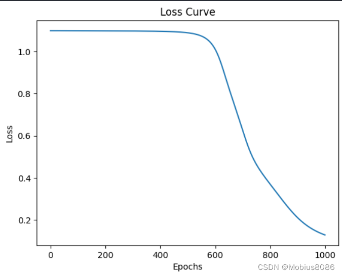
可以看到经过1000轮迭代,最终的准确率到达100%。
回归代码
import numpy as np
from sklearn.model_selection import train_test_split
from sklearn.preprocessing import StandardScaler
import matplotlib.pyplot as plt
from sklearn.datasets import fetch_california_housing
class Layer:
def __init__(self, input_dim, output_dim):
self.W = np.random.randn(input_dim, output_dim) * 0.01
self.b = np.zeros((1, output_dim))
def forward(self, X):
self.Z = np.dot(X, self.W) + self.b
self.A = self.activation(self.Z)
return self.A
def backward(self, dA, X, activation_derivative):
m = X.shape[0]
self.dZ = dA * activation_derivative(self.Z)
self.dW = np.dot(X.T, self.dZ) / m
self.db = np.sum(self.dZ, axis=0, keepdims=True) / m
dA_prev = np.dot(self.dZ, self.W.T)
return dA_prev
def update_parameters(self, learning_rate):
self.W -= learning_rate * self.dW
self.b -= learning_rate * self.db
class ReLULayer(Layer):
def activation(self, Z):
return np.maximum(0, Z)
def activation_derivative(self, Z):
return (Z > 0).astype(float)
class LinearLayer(Layer):
def activation(self, Z):
return Z
def activation_derivative(self, Z):
return np.ones_like(Z)
class NeuralNetwork:
def __init__(self, layer_dims, learning_rate=0.01):
self.layers = []
self.learning_rate = learning_rate
for i in range(len(layer_dims) - 2):
self.layers.append(ReLULayer(layer_dims[i], layer_dims[i + 1]))
self.layers.append(LinearLayer(layer_dims[-2], layer_dims[-1]))
def mean_squared_error(self, y_true, y_pred):
return np.mean((y_true - y_pred) ** 2)
def train(self, X, y, epochs):
loss_history = []
for epoch in range(epochs):
A = X
# Forward propagation
cache = [A]
for layer in self.layers:
A = layer.forward(A)
cache.append(A)
loss = self.mean_squared_error(y, A)
loss_history.append(loss)
# Backward propagation
# 损失函数求导
dA = -(y - A)
for i in reversed(range(len(self.layers))):
layer = self.layers[i]
A_prev = cache[i]
dA = layer.backward(dA, A_prev, layer.activation_derivative)
# Update parameters
for layer in self.layers:
layer.update_parameters(self.learning_rate)
if (epoch + 1) % 100 == 0:
print(f'Epoch {epoch + 1}/{epochs}, Loss: {loss:.4f}')
return loss_history
def predict(self, X):
A = X
for layer in self.layers:
A = layer.forward(A)
return A
housing = fetch_california_housing()
# 导入数据
X = housing.data
y = housing.target.reshape(-1, 1)
# 标准化
scaler_X = StandardScaler()
scaler_y = StandardScaler()
X = scaler_X.fit_transform(X)
y = scaler_y.fit_transform(y)
# 分割数据
X_train, X_test, y_train, y_test = train_test_split(X, y, test_size=0.2, random_state=42)
# 定义并训练神经网络
layer_dims = [X_train.shape[1], 50, 5, 1] # Example with 2 hidden layers
learning_rate = 0.8
epochs = 1000
nn = NeuralNetwork(layer_dims, learning_rate)
loss_history = nn.train(X_train, y_train, epochs)
# 预测和评估
train_predictions = nn.predict(X_train)
test_predictions = nn.predict(X_test)
train_mse = nn.mean_squared_error(y_train, train_predictions)
test_mse = nn.mean_squared_error(y_test, test_predictions)
print(f'Training MSE: {train_mse:.4f}')
print(f'Test MSE: {test_mse:.4f}')
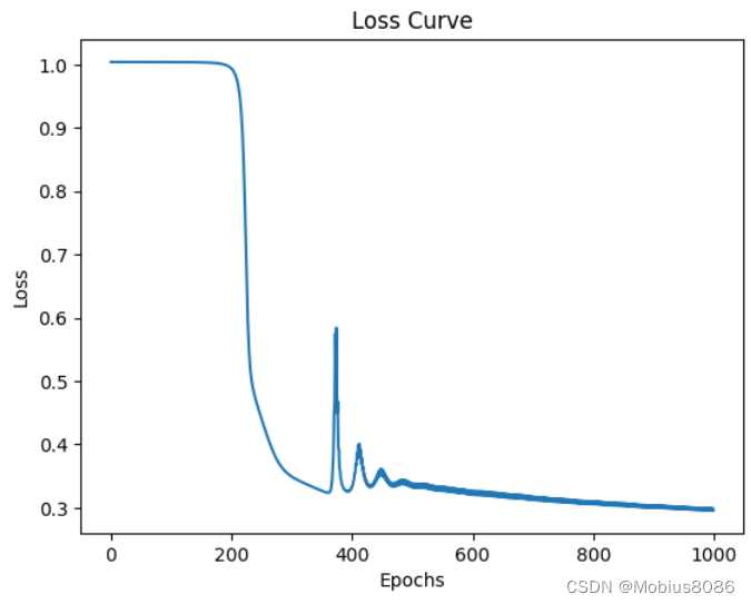
# 绘制损失曲线
plt.plot(loss_history)
plt.xlabel('Epochs')
plt.ylabel('Loss')
plt.title('Loss Curve')
plt.show()
输出
Epoch 100/1000, Loss: 1.0038
Epoch 200/1000, Loss: 0.9943
Epoch 300/1000, Loss: 0.3497
Epoch 400/1000, Loss: 0.3306
Epoch 500/1000, Loss: 0.3326
Epoch 600/1000, Loss: 0.3206
Epoch 700/1000, Loss: 0.3125
Epoch 800/1000, Loss: 0.3057
Epoch 900/1000, Loss: 0.2999
Epoch 1000/1000, Loss: 0.2958
Training MSE: 0.2992
Test MSE: 0.3071