matlab:有限差分求解纳维尔(Navier)边界的双调和(Biharmonic)方程,边值为零

news2025/10/31 23:28:10

我们考虑如下形式的双调和方程的数值解
在这里插入图片描述
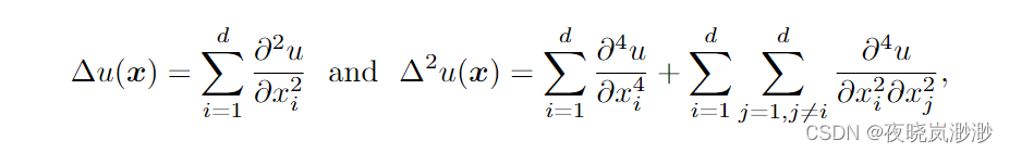
其中，Ω是欧氏空间中的多边形或多面体域，在其中，d为维度，具有分段利普希茨边界，满足内部锥条件，f(x) ∈ L2(Ω)是给定的函数，∆是标准的拉普拉斯算子。算子∆u(x)和∆2u(x)表示为

巧妙地将双调和方程（1.1）分解为两个Possion方程，传统的数值方法如有限元法（FEM）和有限差分法（FDM）在计算资源和时间复杂度较小的情况下表现良好。通过引入辅助变量w = −∆u，可以将四阶方程（1.1）重写为一对二阶方程：
在这里插入图片描述
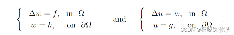
或者引入变量w = ∆u，得到

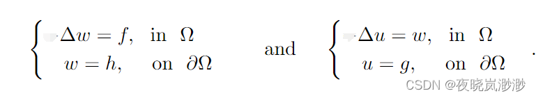
那么，我们的目标为寻找一对函数（w，u），而不是找到原始问题（1.1）的解。如下我们以g=0和h=0为例，利用五点中心差分求解上面的双调和方程。

%%%%%%%%%%%%%%%%%%%%%%%%%%%%%%%%%%%%%%%%%%%%%%%%%%%%%%%%%%%%%
%%%%          Matrix method for Biharmonic Equation      %%%%
%%%     u_{xxxx} + u_{yyyy} + 2*u_{xx}*u_{yy} = f(x, y)  %%%%
%%%           Omega = 0 < x < 1, 0 < y < 1               %%%%
%%%              u(x, y) = 0 on boundary,                %%%%  
%%%  Exact soln: u(x, y) = sin(pi*x)*sin(pi*y)           %%%%
%%%        Here f(x, y) = 4*pi^4*sin(pi*x)*sin(pi*y);   %%%%
%%%        Course:    Ye Xiao Lan on 04.01 2024         %%%% 
%%%%%%%%%%%%%%%%%%%%%%%%%%%%%%%%%%%%%%%%%%%%%%%%%%%%%%%%%%%%%

clear all
clc
close all

ftsz = 20;

x_l = -1.0;
x_r = 1.0;
y_b = -1.0;
y_t = 1.0;

q = 6;
Num = 2^q+1;
NNN = Num*Num;

point_num2x = Num;
point_num2y = Num;

fside = @(x, y) 4*pi^4*sin(pi*x).*sin(pi*y);
utrue = @(x, y) sin(pi*x).*sin(pi*y);

hx = (x_r-x_l)/point_num2x; 
X = zeros(point_num2x-1,1);
for i=1:point_num2x-1
  X(i) = x_l+i*hx;
end

hy = (y_t-y_b)/point_num2y; 
Y=zeros(point_num2y-1,1);
for i=1:point_num2y-1
  Y(i) = y_b+i*hy;
end
[meshX, meshY] = meshgrid(X, Y);

tic;
Unumberi = FDM2Biharmonic_Couple2Navier_Zero(point_num2x, point_num2y,...
                                                x_l, x_r, y_b, y_t, fside);
fprintf('%s%s%s\n','运行时间:',toc,'s')
U_exact = utrue(meshX, meshY);
meshErr = abs(U_exact - Unumberi);

rel_err = sum(sum(meshErr))/sum(sum(abs(U_exact)));
fprintf('%s%s\n','相对误差:',rel_err)

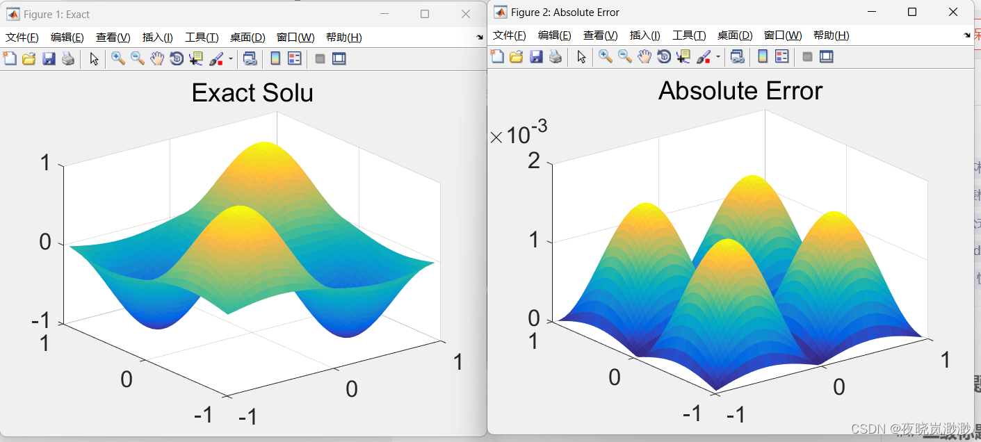
figure('name','Exact')
axis tight;
h = surf(meshX, meshY, U_exact','Edgecolor', 'none');
hold on
title('Exact Solu')
% xlabel('$x$', 'Fontsize', 20, 'Interpreter', 'latex')
% ylabel('$y$', 'Fontsize', 20, 'Interpreter', 'latex')
% zlabel('$Error$', 'Fontsize', 20, 'Interpreter', 'latex')
hold on
set(gca, 'XMinortick', 'off', 'YMinorTick', 'off', 'Fontsize', ftsz);
set(gcf, 'Renderer', 'zbuffer');
hold on
% colorbar;
% caxis([0 0.00012])
hold on

figure('name','Absolute Error')
axis tight;
h = surf(meshX, meshY, meshErr','Edgecolor', 'none');
hold on
title('Absolute Error')
% xlabel('$x$', 'Fontsize', 20, 'Interpreter', 'latex')
% ylabel('$y$', 'Fontsize', 20, 'Interpreter', 'latex')
% zlabel('$Error$', 'Fontsize', 20, 'Interpreter', 'latex')
hold on
set(gca, 'XMinortick', 'off', 'YMinorTick', 'off', 'Fontsize', ftsz);
set(gcf, 'Renderer', 'zbuffer');
hold on
% colorbar;
% caxis([0 0.00012])
hold on

if q==6
    txt2result = 'result2fdm_mesh6.txt';
elseif q==7
    txt2result = 'result2fdm_mesh7.txt';
elseif q==8
    txt2result = 'result2fdm_mesh8.txt';
elseif q==9
    txt2result = 'result2fdm_mesh9.txt';
end

fop = fopen(txt2result, 'wt');

fprintf(fop,'%s%s%s\n','运行时间:',toc,'s');
fprintf(fop,'%s%d\n','内部网格点数目:',Num-1);
fprintf(fop,'%s%s\n','相对误差:',rel_err);

被调用的求解函数如下:

function Uapp = FDM2Biharmonic_Couple2Navier_Zero(Nx, Ny, xleft, xright, ybottom, ytop, fside)
    format long;

    % Define the step sizes and create the grid without boundary points
    hx = (xright-xleft)/Nx; 
    x = zeros(Nx-1,1);
    for ix=1:Nx-1
      x(ix) = xleft+ix*hx;
    end

    hy = (ytop-ybottom)/Ny; 
    y=zeros(Ny-1,1);
    for iy=1:Ny-1
      y(iy) = ybottom+iy*hy;
    end

    % Define the source term
    source_term = fside;

    % Initialize the coefficient matrix A and the right-hand side vector F
    N = (Ny-1)*(Nx-1);
    A = sparse(N,N); 
    FV = zeros(N,1);

    % Loop through each inner grid point, Apply finite difference scheme (central differences)
    hx1 = hx*hx; 
    hy1 = hy*hy; 
    for jv = 1:Ny-1
      for iv=1:Nx-1
        kv = iv + (jv-1)*(Nx-1);
        FV(kv) = fside(x(iv),y(jv));
        A(kv,kv) = -2/hx1 -2/hy1;
        
        %-- x direction --------------
        if iv == 1
            A(kv,kv+1) = 1/hx1;
        else
           if iv==Nx-1
             A(kv,kv-1) = 1/hx1;
           else
            A(kv,kv-1) = 1/hx1;
            A(kv,kv+1) = 1/hx1;
           end
        end
        %-- y direction --------------
        if jv == 1
            A(kv,kv+Nx-1) = 1/hy1;
        else
           if jv==Ny-1
             A(kv,kv-(Nx-1)) = 1/hy1;
           else
              A(kv,kv-(Nx-1)) = 1/hy1;
              A(kv,kv+Nx-1) = 1/hy1;
           end
        end
      end
    end
    V = A\FV;

    B = sparse(N,N); 
    FU = zeros(N,1);

    % Loop through each inner grid point, Apply finite difference scheme (central differences)
    for ju = 1:Ny-1
      for iu=1:Nx-1
        ku = iu + (ju-1)*(Nx-1);
        FV(ku) = V(ku);
        B(ku,ku) = -2/hx1 -2/hy1;
        
        %-- x direction --------------
        if iu == 1
            B(ku,ku+1) = 1/hx1;
        else
           if iu==Nx-1
             B(ku,ku-1) = 1/hx1;
           else
            B(ku,ku-1) = 1/hx1;
            B(ku,ku+1) = 1/hx1;
           end
        end
        %-- y direction --------------
        if ju == 1
            B(ku,ku+Nx-1) = 1/hy1;
        else
           if ju==Ny-1
             B(ku,ku-(Nx-1)) = 1/hy1;
           else
              B(ku,ku-(Nx-1)) = 1/hy1;
              B(ku,ku+Nx-1) = 1/hy1;
           end
        end
      end
    end
    
    U = B\FV;
    %--- Transform back to (i,j) form to plot the solution ---
    j = 1;
    for k=1:N
      i = k - (j-1)*(Nx-1) ;
      Uapp(i,j) = U(k);
      j = fix(k/(Nx-1)) + 1;
    end
end