数据及代码链接见文末
论文解析:Star GAN论文解析-CSDN博客
1.测试模块效果与实验分析
测试数据需要准备两个文件夹src(源)和ref(目标),这两个文件夹下的文件夹名称代表各个domain。

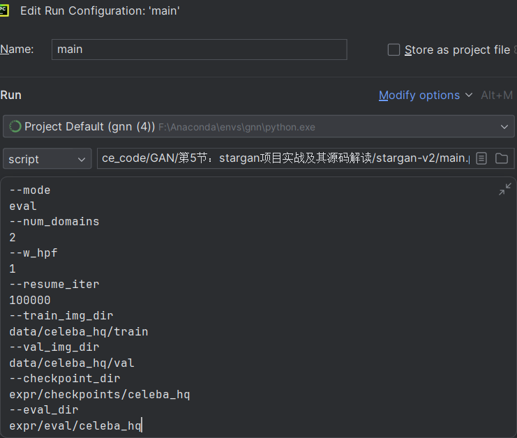
运行测试模块:
python main.py --mode eval --num_domains 2 --w_hpf 1 \
               --resume_iter 100000 \
               --train_img_dir data/celeba_hq/train \
               --val_img_dir data/celeba_hq/val \
               --checkpoint_dir expr/checkpoints/celeba_hq \
               --eval_dir expr/eval/celeba_hq
或者指定参数:
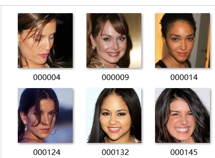
2.项目配置与数据源下载
以人脸数据集为例,数据集下包含训练集和验证集,训练集和测试集下的文件夹代表一个一个domain

需要注意的是,数据集是做过特殊处理的,里面的人脸是对齐的,如果要训练自己的数据集,也需要做类似的处理
环境配置:
- 安装pytorch,默认为1.4版本,比1.4版本高也行
- pip install ffmpeg
-
pip install opencv-python
-
pip install scikit-image
-
pip install pillow
- pip install scipy
- pip install tqdm
- pip install munch
常用参数
模型与损失函数相关
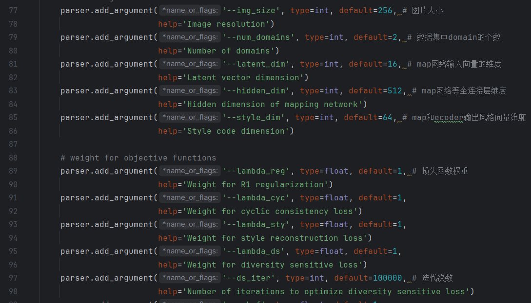
batch size

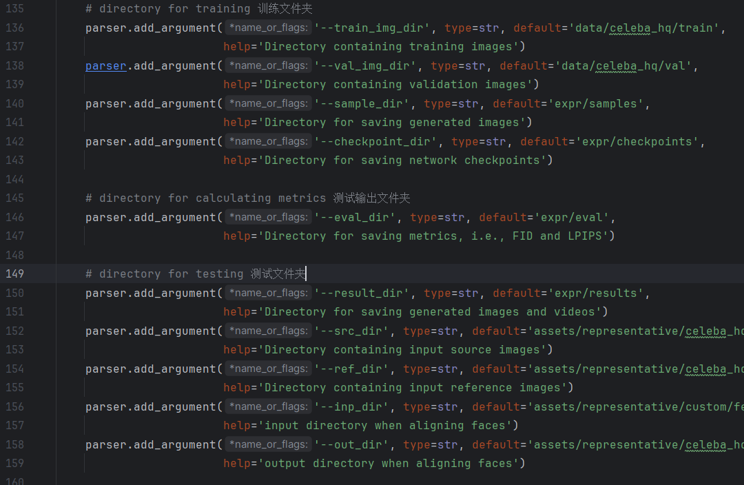
训练和测试输入与测试输出文件夹路径
3.整体流程
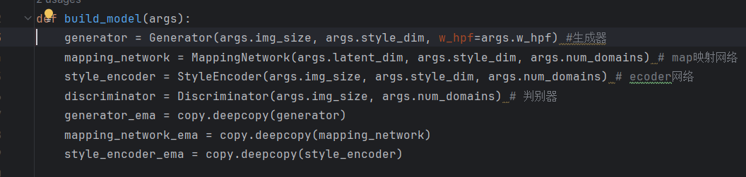
整个网络有四个网络组成,生成器、map映射网络、ecoder、判别器。
- 生成网络,即对输入图像生成一张给定风格的图像
- 映射网络,随机初始化一个向量,通过全连接层得到对应风格的转化向量。
- ecoder:直接将图像编码为对应风格的向量
- 判别器:对于输入图像,为每一种风格判断真假
(1)生成器
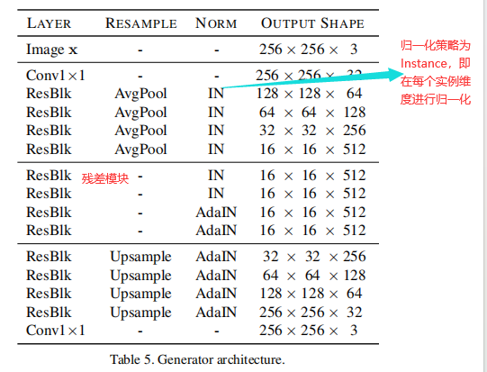
生成器生成特定风格的图像,生成器有U-net结构的网络堆叠而成,即先下采样,在上采样。此处的归一化策略采取Instance norm,即在实例维度进行归一化。并使用残差模块
代码
class Generator(nn.Module):
    def __init__(self, img_size=256, style_dim=64, max_conv_dim=512, w_hpf=1):
        super().__init__()
        dim_in = 2**14 // img_size
        self.img_size = img_size
        self.from_rgb = nn.Conv2d(3, dim_in, 3, 1, 1) #(in_channels,out_channels,kernel_size,stride,padding)
        self.encode = nn.ModuleList()
        self.decode = nn.ModuleList()
        self.to_rgb = nn.Sequential(
            nn.InstanceNorm2d(dim_in, affine=True), # 在每个实例维度进行归一化
            nn.LeakyReLU(0.2),
            nn.Conv2d(dim_in, 3, 1, 1, 0))

        # down/up-sampling blocks
        repeat_num = int(np.log2(img_size)) - 4
        if w_hpf > 0:
            repeat_num += 1
        for _ in range(repeat_num):
            dim_out = min(dim_in*2, max_conv_dim)
            self.encode.append(
                ResBlk(dim_in, dim_out, normalize=True, downsample=True))
            self.decode.insert(
                0, AdainResBlk(dim_out, dim_in, style_dim,
                               w_hpf=w_hpf, upsample=True))  # stack-like
            dim_in = dim_out

        # bottleneck blocks
        for _ in range(2):
            self.encode.append(
                ResBlk(dim_out, dim_out, normalize=True)) # 残差模块
            self.decode.insert(
                0, AdainResBlk(dim_out, dim_out, style_dim, w_hpf=w_hpf))

        if w_hpf > 0:
            device = torch.device(
                'cuda' if torch.cuda.is_available() else 'cpu')
            self.hpf = HighPass(w_hpf, device)

    def forward(self, x, s, masks=None):
        x = self.from_rgb(x)
        cache = {}
        for block in self.encode:
            if (masks is not None) and (x.size(2) in [32, 64, 128]):
                cache[x.size(2)] = x
            x = block(x)
        for block in self.decode:
            x = block(x, s)
            if (masks is not None) and (x.size(2) in [32, 64, 128]):
                mask = masks[0] if x.size(2) in [32] else masks[1]
                mask = F.interpolate(mask, size=x.size(2), mode='bilinear')
                x = x + self.hpf(mask * cache[x.size(2)])
        return self.to_rgb(x)
(2)Map映射网络
map网络将随机初始化的隐向量转变为风格向量。 map映射网络主要由全连接层构成
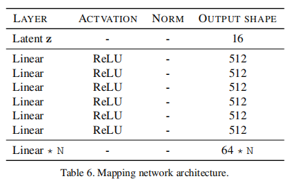
代码实现:
class MappingNetwork(nn.Module):
    def __init__(self, latent_dim=16, style_dim=64, num_domains=2):
        super().__init__()
        layers = []
        layers += [nn.Linear(latent_dim, 512)]
        layers += [nn.ReLU()]
        for _ in range(3):
            layers += [nn.Linear(512, 512)]
            layers += [nn.ReLU()]
        self.shared = nn.Sequential(*layers)

        self.unshared = nn.ModuleList()
        for _ in range(num_domains):
            self.unshared += [nn.Sequential(nn.Linear(512, 512),
                                            nn.ReLU(),
                                            nn.Linear(512, 512),
                                            nn.ReLU(),
                                            nn.Linear(512, 512),
                                            nn.ReLU(),
                                            nn.Linear(512, style_dim))]

    def forward(self, z, y):
        h = self.shared(z)
        out = []
        for layer in self.unshared:
            out += [layer(h)]
        out = torch.stack(out, dim=1)  # (batch, num_domains, style_dim)
        idx = torch.LongTensor(range(y.size(0))).to(y.device)
        s = out[idx, y]  # (batch, style_dim)
        return s
(3)判别器
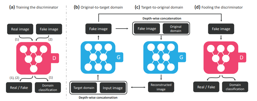
判别器用于判断生成图片和原始图片的真假。其也是由残差模块堆叠而成。具体来说,生成图片向量预测接近于1,原始图片预测接近于0。但是,与传统的生成器不同,这里的生成器对于每一个domain都要预测。
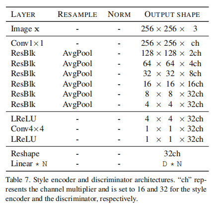
(4)style ecoder
style ecoder为生成图片预测对应的风格向量。其输入为生成的图片,输出为风格向量。风格向量应该与生成这张图片时生成器输入的风格向量非常相近。其网络结构也与判别器相同。
4. 损失函数
1.Style reconstruction
首先,在使用生成网络生成图片时,我们会输入一张图片和对应风格的向量s,然后生成得到对应风格的图片。在得到生成图片后,我们再使用ecoder将生成图片编码为对应风格的向量s'。很显然,我们希望s和s'足够接近。

2.Style diversification(多样性损失)
首先,初始化2组向量z1和z2,然后经过map网络得到对应风格的编码s1和s2,很显然,s1和s2是不同的,我们现在希望根据s1和s2生成的结果差异越大越好,差异越大,多样性越高。即损失函数越大越好

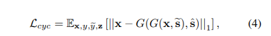
3.Preserving source characteristics
可以理解为一种重构损失,我们希望生成的结果还是同一个人,因此,对于生成图片还原回去要与原来的输入图片足够接近。
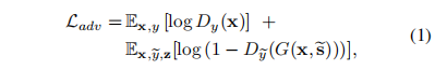
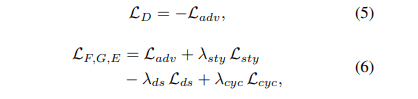
4.Adversarial objective
即判别器损失,原始图片预测接近于1,而生成图像预测接近于0
总损失为上述损失的加权和
数据及代码链接:链接:https://pan.baidu.com/s/1aNlghgo6mtD4iWqNgMOWOQ?pwd=s206
提取码:s206