过拟合和欠拟合

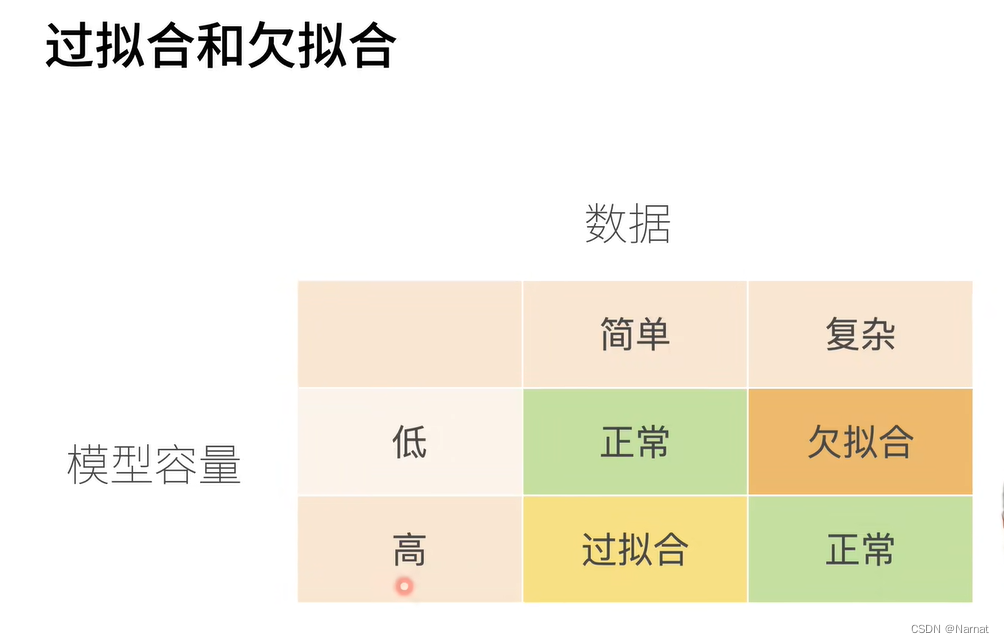
过拟合和欠拟合是训练模型中常会发生的事，如所要识别手势过于复杂，如五角星手势，那就需要更改高级更复杂的模型去训练，若用比较简单模型去训练，就会导致模型未能抓住手势的全部特征，那简单模型估计只能抓住五角星的其中一个角做特征，那么这个简单模型很可能就会将三角形与五角星混淆，这就是所谓欠拟合

若用识别五角星的复杂模型去识别三角形也是不行的，模型会过拟合，即学习了过多不重要的部分，可能会把三角形每条边所画的时间也当作学习的内容，即便我们人知道什么时候画哪条边都无所谓。

过拟合和欠拟合的表现都是模型的识别精度不够，所以要想判断模型是过拟合还是欠拟合，除了理论还是要多调试

如：

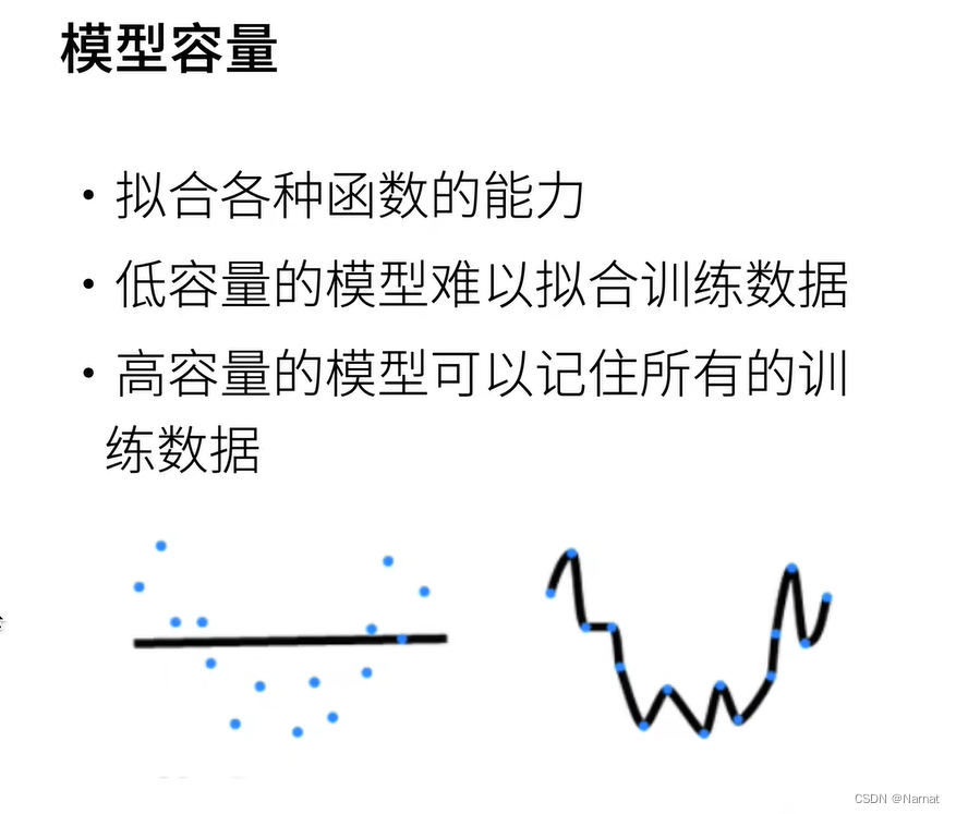
合适的模型应该是抛物线，上述左边是欠拟合，右边是过拟合

训练集和测试集

值得注意的是训练集和测试集必须是分开的，训练模型用训练集，一定不能让测试集污染模型

模型过拟的特征即对见过的数据集表现非常好，而对从未见过的模型表现非常差，若不把训练，测试集完全分开，最后的模型过拟合将无法被发现

实例：

完整代码：

import math
import torch
from torch import nn
from d2l import torch as d2l
import matplotlib.pyplot as plt

# 生成随机的数据集
max_degree = 20  # 多项式的最大阶数
n_train, n_test = 100, 100  # 训练和测试数据集大小
true_w = torch.zeros(max_degree)
true_w[0:4] = torch.Tensor([5, 1.2, -3.4, 5.6])

# 生成特征
features = torch.randn((n_train + n_test, 1))
permutation_indices = torch.randperm(features.size(0))
# 使用随机排列的索引来打乱features张量（原地修改）
features = features[permutation_indices]
poly_features = torch.pow(features, torch.arange(max_degree).reshape(1, -1))
for i in range(max_degree):
    poly_features[:, i] /= math.gamma(i + 1)

# 生成标签
labels = torch.matmul(poly_features, true_w)
labels += torch.normal(0, 0.1, size=labels.shape)


# 以下是你原来的训练函数，没有修改
def evaluate_loss(net, data_iter, loss):
    metric = d2l.Accumulator(2)
    for X, y in data_iter:
        out = net(X)
        y = y.reshape(out.shape)
        l = loss(out, y)
        metric.add(l.sum(), l.numel())
    return metric[0] / metric[1]


def train(train_features, test_features, train_labels, test_labels,
          num_epochs=400):
    loss = nn.MSELoss()
    input_shape = train_features.shape[-1]
    net = nn.Sequential(nn.Linear(input_shape, 1, bias=False))
    batch_size = min(10, train_labels.shape[0])

    train_iter = d2l.load_array((train_features, train_labels.reshape(-1, 1)),
                                batch_size)
    test_iter = d2l.load_array((test_features, test_labels.reshape(-1, 1)),
                               batch_size, is_train=False)
    trainer = torch.optim.SGD(net.parameters(), lr=0.01)

    # 用于存储训练和测试损失的列表
    train_losses = []
    test_losses = []

    for epoch in range(num_epochs):
        train_loss, train_acc = d2l.train_epoch_ch3(net, train_iter, loss, trainer)
        test_loss = evaluate_loss(net, test_iter, loss)

        # 将当前的损失值添加到列表中
        train_losses.append(train_loss)
        test_losses.append(test_loss)

        print(f"Epoch {epoch + 1}/{num_epochs}:")
        print(f"  训练损失： {train_loss:.4f}, 测试损失： {test_loss:.4f}")
    print(net[0].weight)
    # 假设 train_losses 和 test_losses 是已经计算出的损失值列表
    plt.figure(figsize=(10, 6))
    plt.plot(train_losses, label='train', color='blue', linestyle='-', marker='.')
    plt.plot(test_losses, label='test', color='purple', linestyle='--', marker='.')
    plt.xlabel('epoch')
    plt.ylabel('loss')
    plt.title('Loss over Epochs')
    plt.legend()
    plt.grid(True)
    plt.ylim(0, 100)  # 设置y轴的范围从0.01到100
    plt.show()


# 选择多项式特征中的前4个维度
train(poly_features[:n_train, :4], poly_features[n_train:, :4],
      labels[:n_train], labels[n_train:])

分部讲解如下：

问题实例：

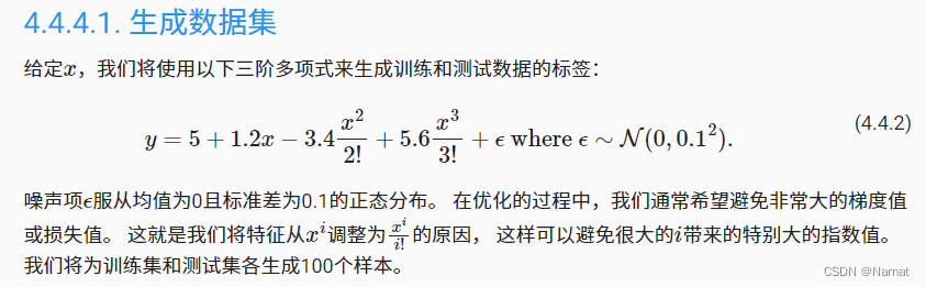
产生高斯分布随机数x并按上述式子生成训练集和验证集y，并对生成的y再添加一些杂音处理
注意：训练集一定要打乱，不要排序，排序会让训练效果大打折扣，如果训练数据是按照某种特定顺序排列的，那么模型可能会学习到这种顺序并在这个过程中引入偏差，导致模型在未见过的新数据上的泛化能力下降，打乱训练集的目的通常是为了防止模型学习到训练数据中的任何顺序依赖性，这样可以提高模型在随机或未见过的新数据上的泛化能力。

# 生成随机的数据集
max_degree = 20  # 多项式的最大阶数
n_train, n_test = 100, 100  # 训练和测试数据集大小
true_w = torch.zeros(max_degree)
true_w[0:4] = torch.Tensor([5, 1.2, -3.4, 5.6])

# 生成特征
features = torch.randn((n_train + n_test, 1))
permutation_indices = torch.randperm(features.size(0))
# 使用随机排列的索引来打乱features张量（原地修改）
features = features[permutation_indices]
poly_features = torch.pow(features, torch.arange(max_degree).reshape(1, -1))
for i in range(max_degree):
    poly_features[:, i] /= math.gamma(i + 1)

# 生成标签
labels = torch.matmul(poly_features, true_w)
labels += torch.normal(0, 0.1, size=labels.shape)

计算损失函数，并不会更新迭代模型，所以用他来测试模型测试集损失

def evaluate_loss(net, data_iter, loss):
    metric = d2l.Accumulator(2)
    for X, y in data_iter:
        out = net(X)
        y = y.reshape(out.shape)
        l = loss(out, y)
        metric.add(l.sum(), l.numel())
    return metric[0] / metric[1]

训练函数，将X和对应y放在一起，即是进行模型迭代更新，又能计算模型训练损失，测试损失并绘制相应图形

def train(train_features, test_features, train_labels, test_labels,
          num_epochs=400):
    loss = nn.MSELoss()  # 默认取平均损失
    input_shape = train_features.shape[-1]  # 模型大小取train_features最后一项大小
    net = nn.Sequential(nn.Linear(input_shape, 1, bias=False))
    batch_size = min(10, train_labels.shape[0])  # 整体数据集分成<= 10批次

    train_iter = d2l.load_array((train_features, train_labels.reshape(-1, 1)),
                                batch_size)
    test_iter = d2l.load_array((test_features, test_labels.reshape(-1, 1)),
                               batch_size, is_train=False)
    trainer = torch.optim.SGD(net.parameters(), lr=0.01)  # 梯度下降算法

    # 用于存储训练和测试损失的列表
    train_losses = []
    test_losses = []

    for epoch in range(num_epochs):
        train_loss, train_acc = d2l.train_epoch_ch3(net, train_iter, loss, trainer)  # 训练迭代模型
        test_loss = evaluate_loss(net, test_iter, loss)

        # 将当前的损失值添加到列表中
        train_losses.append(train_loss)
        test_losses.append(test_loss)

        print(f"Epoch {epoch + 1}/{num_epochs}:")
        print(f"  训练损失： {train_loss:.4f}, 测试损失： {test_loss:.4f}")
    print(net[0].weight)  # 输出训练好的模型
    # 假设 train_losses 和 test_losses 是已经计算出的损失值列表
    plt.figure(figsize=(10, 6))
    plt.plot(train_losses, label='train', color='blue', linestyle='-', marker='.')
    plt.plot(test_losses, label='test', color='purple', linestyle='--', marker='.')
    plt.xlabel('epoch')
    plt.ylabel('loss')
    plt.title('Loss over Epochs')
    plt.legend()
    plt.grid(True)
    plt.ylim(0, 100)  # 设置y轴的范围从0.01到100
    plt.show()

主函数

# 选择多项式特征中的前4个维度
train(poly_features[:n_train, :4], poly_features[n_train:, :4],
      labels[:n_train], labels[n_train:])

利用上述实例验证欠拟合和过拟合以及正常拟合

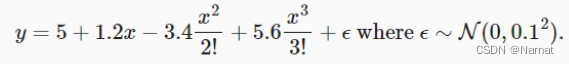
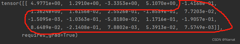
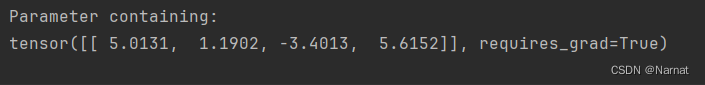
上述函数对应真正的模型为：

true_w[0:4] = torch.Tensor([5, 1.2, -3.4, 5.6])

当然还有一些杂质，可忽略

那么可知预训练模型取四个维度就能做到正常拟合，而取二十个维度就是过拟合，取四个以下维度就是欠拟合

过拟合即取二十维度效果：

可以看出损失在下降到最低点的时候还会有上升

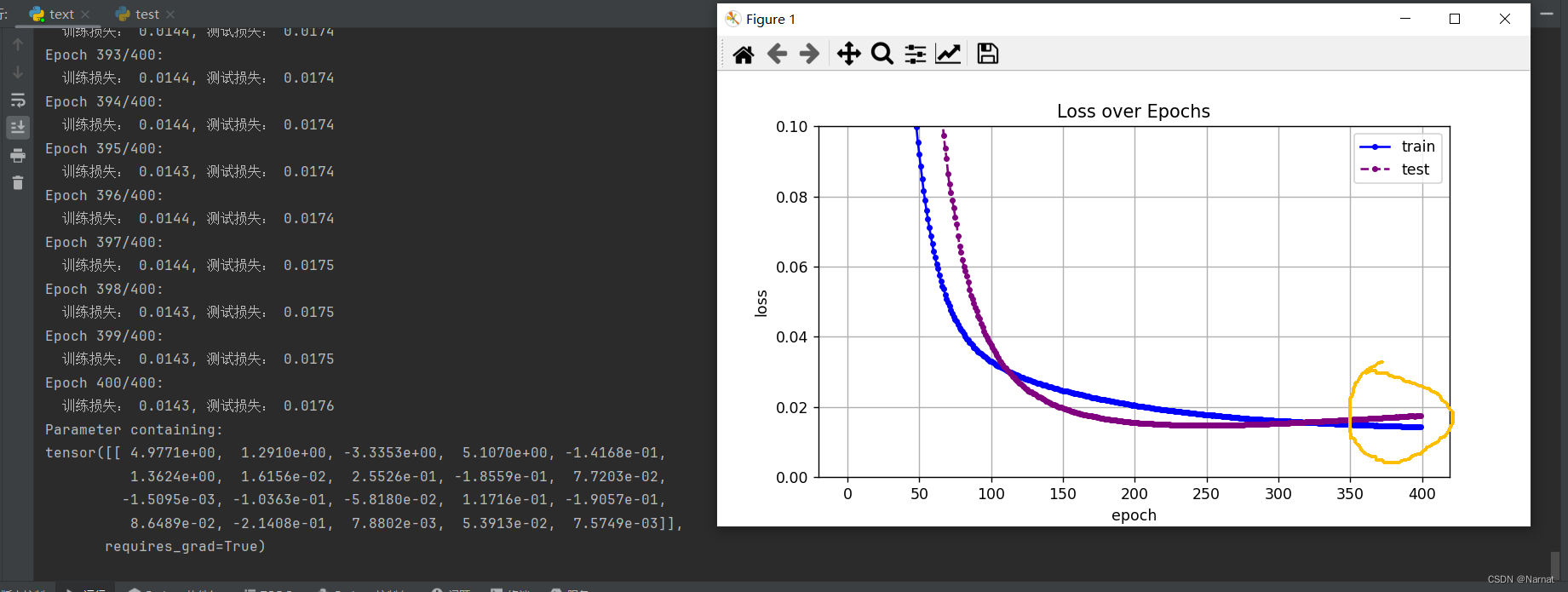
这是因为学完主要四个维度后又将本应是0的维度也学习了，也就是学习了无用的杂质。

欠拟合二维度模型效果：

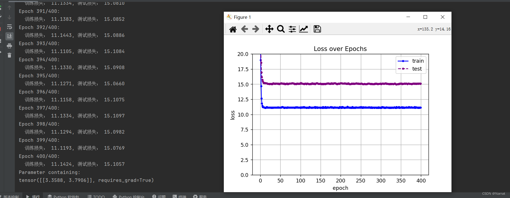
损失很大,这也是没办法，毕竟还有很多重要维度没有学习上，本质上是模型过小

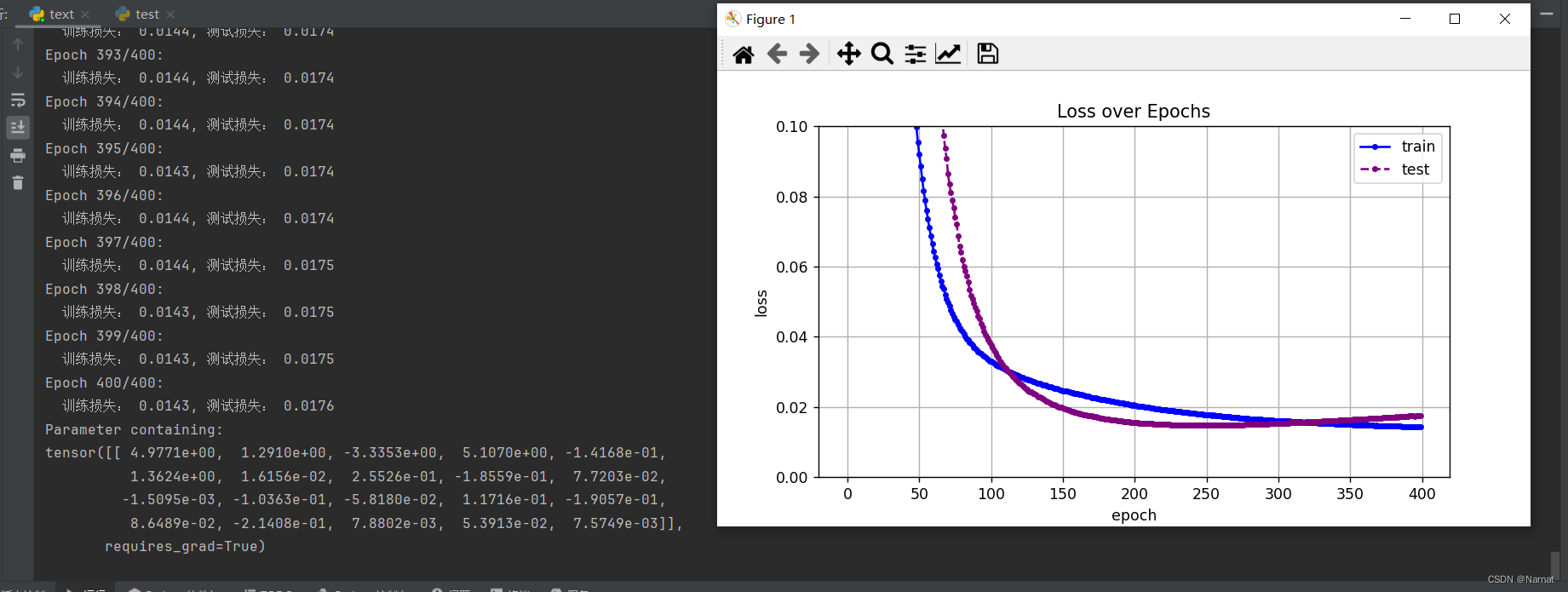
正常拟合四维度模型效果：

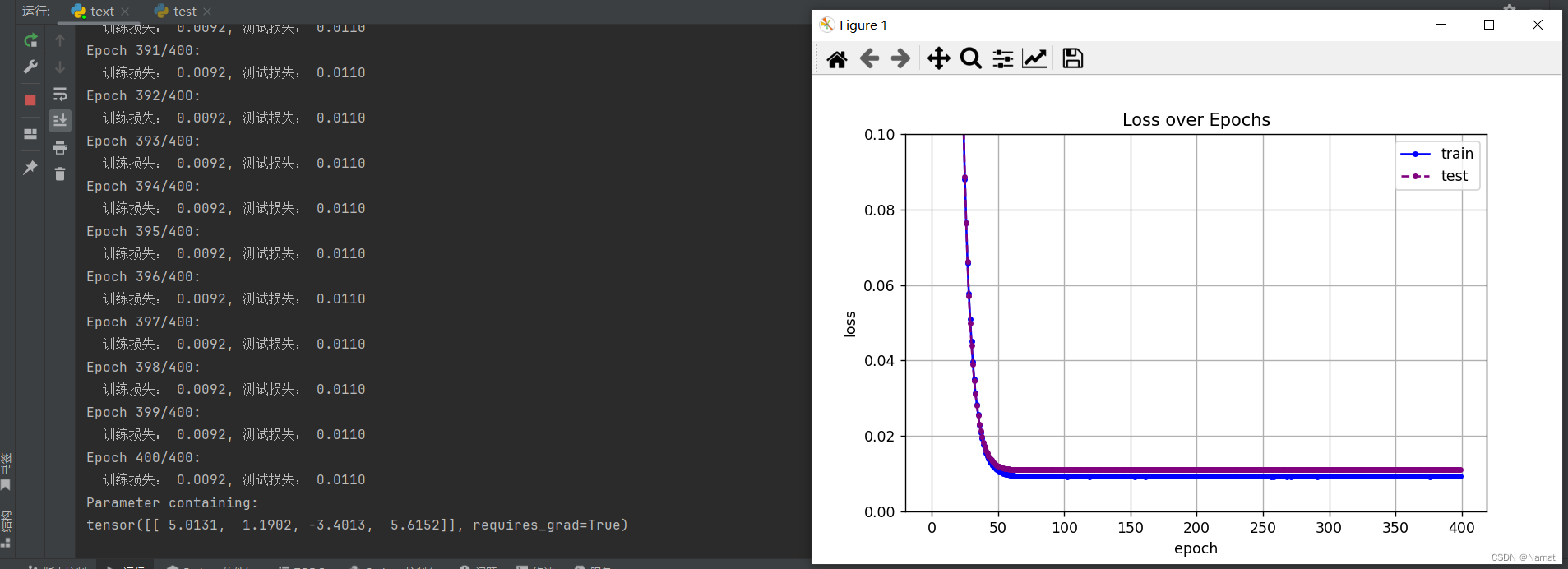
正常拟合的模型在损失到达最低点后便不再上升，训练出来的模型与真实数据也及其接近

正常拟合才是我们训练模型的期望状态