线性回归
线性回归是一种监督学习方法,用于建立因变量与一个或多个自变量之间的关系。线性回归的目标是找到一条直线,使得所有数据点到这条直线的距离之和最小。
线性回归的基本形式如下:
y = β 0 + β 1 x 1 + β 2 x 2 + . . . + β n x n + ϵ y = \beta_0 + \beta_1x_1 + \beta_2x_2 + ... + \beta_nx_n + \epsilon y=β0+β1x1+β2x2+...+βnxn+ϵ
其中, y y y 是因变量, x 1 , x 2 , . . . , x n x_1, x_2, ..., x_n x1,x2,...,xn 是自变量, β 0 , β 1 , . . . , β n \beta_0, \beta_1, ..., \beta_n β0,β1,...,βn 是参数, ϵ \epsilon ϵ 是误差项。
线性回归的目标是通过最小化以下的均方误差(Mean Squared Error, MSE)来求解参数 β \beta β:
M S E = 1 N ∑ i = 1 N ( y i − ( β 0 + β 1 x i 1 + β 2 x i 2 + . . . + β n x i n ) ) 2 MSE = \frac{1}{N}\sum_{i=1}^{N}(y_i - (\beta_0 + \beta_1x_{i1} + \beta_2x_{i2} + ... + \beta_nx_{in}))^2 MSE=N1i=1∑N(yi−(β0+β1xi1+β2xi2+...+βnxin))2
其中,
N
N
N 是样本数量,
y
i
y_i
yi 是第
i
i
i 个样本的因变量值,
x
i
j
x_{ij}
xij 是第
i
i
i 个样本的第
j
j
j 个自变量值。
这个问题可以转化为一个优化问题,通过梯度下降等方法求解。具体的步骤如下:
- 初始化参数 β \beta β;
- 计算当前参数下的均方误差;
- 根据均方误差的梯度,更新参数 β \beta β;
- 重复步骤2和3,直到收敛。
在这个过程中,参数 β \beta β 的更新规则如下:
β = β − α ∇ M S E \beta = \beta - \alpha\nabla MSE β=β−α∇MSE
其中, α \alpha α 是学习率, ∇ M S E \nabla MSE ∇MSE 是均方误差关于 β \beta β 的梯度。
工具函数
对数据进行标准化
在线性回归中,数据标准化是一个非常重要的步骤,它可以使得不同的特征在模型中具有相同的重要性。数据标准化的一般步骤如下:
- 计算每个特征的均值 μ \mu μ 和标准差 σ \sigma σ:
μ = 1 N ∑ i = 1 N x i \mu = \frac{1}{N}\sum_{i=1}^{N}x_i μ=N1i=1∑Nxi
σ = 1 N ∑ i = 1 N ( x i − μ ) 2 \sigma = \sqrt{\frac{1}{N}\sum_{i=1}^{N}(x_i - \mu)^2} σ=N1i=1∑N(xi−μ)2
其中, N N N 是样本数量, x i x_i xi 是第 i i i 个样本的特征值。
- 将每个特征的值减去均值并除以标准差,得到标准化后的特征值:
z i = x i − μ σ z_i = \frac{x_i - \mu}{\sigma} zi=σxi−μ
其中, z i z_i zi 是第 i i i 个样本的标准化后的特征值。
这样,我们就得到了标准化后的数据,其中每个特征的均值为0,标准差为1。这样可以保证不同的特征在模型中具有相同的重要性,而不会被大的特征值所主导。
def prepare_data(data, normalize_data=True):
    # 标准化特征矩阵(可选)
    if normalize_data:
        features_mean = np.mean(data, axis=0)    #特征的平均值
        features_dev = np.std(data, axis=0)      #特征的标准偏差
        features = (data - features_mean) / features_dev    #标准化数据
    else:
        features_mean = None
        features_dev = None

    ...
为数据集增加偏置项特征
在线性回归模型中,我们通常在数据集前面加一列1,这是因为我们需要一个偏置项(也称为截距项)。偏置项是一个常数,它表示当所有特征都等于0时的预期输出。在实际应用中,偏置项通常被添加到模型中,以便模型可以预测当所有特征都等于0时的输出。
在数学表达式中,线性回归模型可以写为:
y
^
=
θ
0
+
θ
1
x
1
+
θ
2
x
2
+
.
.
.
+
θ
n
x
n
\hat{y} = \theta_0 + \theta_1x_1 + \theta_2x_2 + ... + \theta_nx_n
y^=θ0+θ1x1+θ2x2+...+θnxn
其中,
y
^
\hat{y}
y^是预测的目标变量,
x
1
,
x
2
,
.
.
.
,
x
n
x_1, x_2, ..., x_n
x1,x2,...,xn是特征变量,
θ
0
,
θ
1
,
.
.
.
,
θ
n
\theta_0, \theta_1, ..., \theta_n
θ0,θ1,...,θn是模型的参数。
在这个公式中,
θ
0
\theta_0
θ0就是偏置项。当所有的
x
i
x_i
xi都等于0时,
y
^
\hat{y}
y^就等于
θ
0
\theta_0
θ0。
我们通常将数据集的特征矩阵与一个全1的向量进行水平堆叠(horizontal stacking),以此来添加偏置项。例如,如果我们的特征矩阵是
X
X
X,那么我们可以这样添加偏置项:
这样,我们就得到了一个新的特征矩阵,其中第一列是全1的向量,表示偏置项。
    # 为特征添加偏置项
    data_processed = np.hstack((np.ones((features.shape[0], 1)), features)).T
    # 返回处理后的数据
    return data_processed, features_mean, features_dev
预测结果评估函数
获取评分和分级以便可视化处理
def get_predict_score(predict_table):
    score_table = []
    pass_count = 0
    for pair in predict_table:
        if (abs(pair[0] - pair[1]) / pair[1] < 0.1):
            score_table.append("good")
            pass_count += 1
        elif (abs(pair[0] - pair[1]) / pair[1] < 0.4):
            score_table.append("around")
            pass_count += 0.8
        else:
            score_table.append("bad")
    accuracy = pass_count / len(predict_table)
    return score_table, accuracy
线性回归类
以下的代码位于名为 LinearRegression的类中
初始化
在初始化中获取处理后的数据,并初始化权重向量
def __init__(self, data,labels, normalize_data = True) -> None:
        (data_proccessed,
         features_mean,
         features_dev) = prepare_data(data, normalize_data)
        self.data = data_proccessed
        self.labels = labels
        self.features_mean = features_mean
        self.features_dev = features_dev
        self.normalize_data = normalize_data

        num_features = self.data.shape[0] #特征个数
        self.theta = np.zeros((num_features,1)) #初始化权重向量
训练过程
单步更新权重
首先计算权重和特征的点积,计算预测值
通过最小化以下的均方误差来求解参数
β
\beta
β:
MSE的定义是:
M S E = 1 N ∑ i = 1 N ( y i − ( β 0 + β 1 x i 1 + β 2 x i 2 + . . . + β n x i n ) ) 2 MSE = \frac{1}{N} \sum_{i=1}^{N} (y_i - (\beta_0 + \beta_1x_{i1} + \beta_2x_{i2} + ... + \beta_nx_{in}))^2 MSE=N1i=1∑N(yi−(β0+β1xi1+β2xi2+...+βnxin))2
将 ( β 0 + β 1 x i 1 + β 2 x i 2 + . . . + β n x i n ) (\beta_0 + \beta_1x_{i1} + \beta_2x_{i2} + ... + \beta_nx_{in}) (β0+β1xi1+β2xi2+...+βnxin) 看作一个整体, 对它求偏导,MSE的梯度可以通过以下公式计算:
d
M
S
E
d
θ
=
1
N
∑
i
=
1
N
−
2
(
y
i
−
(
β
0
+
β
1
x
i
1
+
β
2
x
i
2
+
.
.
.
+
β
n
x
i
n
)
)
x
i
j
\frac{dMSE}{d\theta} = \frac{1}{N} \sum_{i=1}^{N} -2 (y_i - (\beta_0 + \beta_1x_{i1} + \beta_2x_{i2} + ... + \beta_nx_{in})) x_{ij}
dθdMSE=N1i=1∑N−2(yi−(β0+β1xi1+β2xi2+...+βnxin))xij
其中,
x
i
j
x_{ij}
xij是第
i
i
i个样本的第
j
j
j个特征的值。
这个公式的意思是,对于每一个样本,我们首先计算预测值和真实值之间的差距,然后乘以这个差距的符号(也就是
−
2
(
y
i
−
(
β
0
+
β
1
x
i
1
+
β
2
x
i
2
+
.
.
.
+
β
n
x
i
n
)
)
-2(y_i - (\beta_0 + \beta_1x_{i1} + \beta_2x_{i2} + ... + \beta_nx_{in}))
−2(yi−(β0+β1xi1+β2xi2+...+βnxin))),再乘以这个特征的值
x
i
j
x_{ij}
xij。这样,我们就得到了每个特征对MSE的贡献。
然后,我们可以使用这个梯度来更新参数theta。在这个函数中,首先计算了预测值和真实值之间的偏差向量delta,然后根据这个偏差向量来更新权重参数theta。
具体来说,这个更新过程是通过以下公式完成的:
θ − = l r ⋅ 1 n u m _ e x a m p l e s ⋅ ( n p . d o t ( d e l t a . T , s e l f . d a t a . T ) ) . T \theta -= lr \cdot \frac{1}{num\_examples} \cdot (np.dot(delta.T, self.data.T)).T θ−=lr⋅num_examples1⋅(np.dot(delta.T,self.data.T)).T
其中,lr是学习率,
n
u
m
_
e
x
a
m
p
l
e
s
num\_examples
num_examples是样本数量,delta是偏差向量,self.data是特征矩阵。这个公式表示,我们把权重参数theta减去学习率乘以偏差向量和特征矩阵的点积的结果,从而实现参数的更新。
def gradient_step(self,lr):
        '''
        梯度下降参数更新,使用矩阵运算
        '''
        num_examples = self.data.shape[1] # 多少行
        prediction = LinearRegression.predict(self.data, self.theta) #每次计算所有样本的预测值,使用矩阵乘法
        delta = prediction - self.labels # 偏差向量
        theta = self.theta
        theta -= lr*(1/num_examples)*(np.dot(delta.T, self.data.T)).T #更新权重
        self.theta = theta #记录当前权重参数
损失函数
首先计算权重和特征的点积,计算预测值
通过最小化以下的均方误差来求解参数
β
\beta
β:
M
S
E
=
1
N
∑
i
=
1
N
(
y
i
−
(
β
0
+
β
1
x
i
1
+
β
2
x
i
2
+
.
.
.
+
β
n
x
i
n
)
)
2
MSE = \frac{1}{N}\sum_{i=1}^{N}(y_i - (\beta_0 + \beta_1x_{i1} + \beta_2x_{i2} + ... + \beta_nx_{in}))^2
MSE=N1i=1∑N(yi−(β0+β1xi1+β2xi2+...+βnxin))2
通过添加表示偏置项的值为1的列得到
M
S
E
=
1
N
∑
i
=
0
N
(
y
i
−
(
β
^
x
i
^
)
)
2
MSE = \frac{1}{N}\sum_{i=0}^{N}(y_i - (\hat{\beta} \hat{x_i}))^2
MSE=N1i=0∑N(yi−(β^xi^))2
其中
(
β
^
x
i
^
)
)
(\hat{\beta} \hat{x_i}))
(β^xi^)) 即是如下代码中的 ‘delta’(
δ
^
\hat{\delta}
δ^),因为涉及向量的平方所以
(
δ
^
)
2
=
(
n
p
.
d
o
t
(
d
e
l
t
a
.
T
,
d
e
l
t
a
)
)
(\hat{\delta})^2 = (np.dot(delta.T, delta))
(δ^)2=(np.dot(delta.T,delta))
def cost_function(self,data,labels):
        num_examples = data.shape[0]
        delta = LinearRegression.predict(self.data, self.theta) - labels #偏差
        cost = (1/2)*np.dot(delta.T, delta) #最小二乘法计算损失
        #print(cost.shape)
        return cost[0][0]
迭代执行梯度下降更新参数
这一部分没什么好说的,还是对迭代次数和学习率两个超参数做一下说明
在线性回归中,学习率(learning rate)和迭代次数(number of iterations)是两个非常重要的超参数,它们直接影响到模型的训练效果。
-
学习率(Learning Rate):学习率决定了每一步梯度下降的步长。如果学习率太大,那么在搜索最优解的过程中可能会“跳过”最优解;如果学习率太小,那么训练过程可能会非常慢,甚至可能陷入局部最优解。因此,选择合适的学习率是非常重要的。
-
迭代次数(Number of Iterations):迭代次数决定了梯度下降的迭代次数。如果迭代次数太少,那么模型可能还没有收敛到最优解;如果迭代次数太多,那么可能会导致过拟合,模型在训练集上的表现很好,但在测试集上的表现很差。因此,选择合适的迭代次数也是非常重要的。
def gradient_desent(self, lr, num_iter):
        cost_history = []
        for _ in range(num_iter): # 在规定的迭代次数里执行训练
            self.gradient_step(lr)
            cost_history.append(self.cost_function(self.data, self.labels)) # 记录损失值,以便可视化展示
        return cost_history
预测
线性回归模型的预测即是将权重向量和特征向量进行点积,有人可能会问偏置项去了哪里,其实偏置项就藏在权重向量的第一个元素里,因为我们在前面处理数据集的时候已经向数据集的开头添加了一列“1”,所以在进行点积的时候,自动就变成了 y i = b i a s ∗ 1 + x i 1 w i 1 + x i 2 w i 2 + . . . + x i n w i n y_i = bias*1 + x_{i1}w_{i1} + x_{i2}w_{i2} +... + x_{in}w_{in} yi=bias∗1+xi1wi1+xi2wi2+...+xinwin
def predict_test(self, data):
        data_proccessed = prepare_data(data, self.normalize_data)[0]
        prediction = LinearRegression.predict(data_proccessed, self.theta)
        return prediction
    @staticmethod
    def predict(data, theta):
        prediction = np.dot(data.T, theta) #特征值和权重参数做点积,计算预测值
        return prediction
训练,预测和可视化展示部分
没什么好说的,主要就是处理数据集和可视化展示
import pandas as pd
import matplotlib.pyplot as plt
def main():
    data_file = "J:\\MachineLearning\\数据集\\housing.data"
    data = pd.read_csv(data_file, sep="\s+").sample(frac=1).reset_index(drop=True)
    train_data = data.sample(frac=0.8)
    test_data = data.drop(train_data.index)
    input_param_index = 'NOX'
    output_param_index = 'MEDV'
    x_train = train_data[input_param_index].values
    y_train = train_data[output_param_index].values
    x_test = test_data[input_param_index].values
    y_test = test_data[output_param_index].values

    x_train = train_data.iloc[:, :13].values
    y_train = train_data[output_param_index].values.reshape(len(x_train),1)
    x_test = test_data.iloc[:, :13].values
    y_test = test_data[output_param_index].values.reshape(len(test_data),1)
    print(x_train.shape)
    print(y_train.shape)

    linearReg = LinearRegression(x_train, y_train)
    train_theta, loss_history = linearReg.train(0.0001, 50000)
    fomula = 'Y = '
    index = 0
    for w in np.round(train_theta, 2)[1:]:
        fomula += "{}{}X{}".format(" + " if w >=0 else " - " if index != 0 else "", float(abs(w[0])), index)
        index += 1
    fomula += "{}{}".format(" + " if train_theta[0] >= 0 else "-", round(float(abs(train_theta[0][0])), 2))
    print(fomula)
    print(train_theta.shape)
    plt.plot(loss_history)
    plt.show()

    predic_result = np.round(linearReg.predict_test(x_test), 2)
    predict_table = np.column_stack((predic_result, y_test))
    score, accuracy = get_predict_score(predict_table)
    print("Accuracy is {}".format(accuracy))
    color_table = {"good": "green", "around":"yellow", "bad": "red"}
    #print(predic_result)
    fig, ax = plt.subplots()
    table = ax.table(cellText = predict_table, loc = 'center')
    for i, cell in enumerate(table._cells.values()):
        color_index = int(i / 2)
        cell.set_facecolor(color_table[score[color_index]])
    ax.axis("off")
    plt.show()
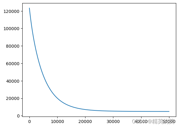
运行结果
损失值变化
得到的展开式
Y
=
0.59
X
0
+
0.48
X
1
−
0.55
X
2
+
0.89
X
3
−
1.18
X
4
+
3.23
X
5
+
0.0
X
6
−
2.2
X
7
+
1.0
X
8
−
0.45
X
9
−
1.82
X
1
0
+
0.82
X
1
1
−
3.66
X
1
2
+
22.67
Y = 0.59X_0 + 0.48X_1 - 0.55X_2 + 0.89X_3 - 1.18X_4 + 3.23X_5 + 0.0X_6 - 2.2X_7 + 1.0X_8 - 0.45X_9 - 1.82X_10 + 0.82X_11 - 3.66X_12 + 22.67
Y=0.59X0+0.48X1−0.55X2+0.89X3−1.18X4+3.23X5+0.0X6−2.2X7+1.0X8−0.45X9−1.82X10+0.82X11−3.66X12+22.67
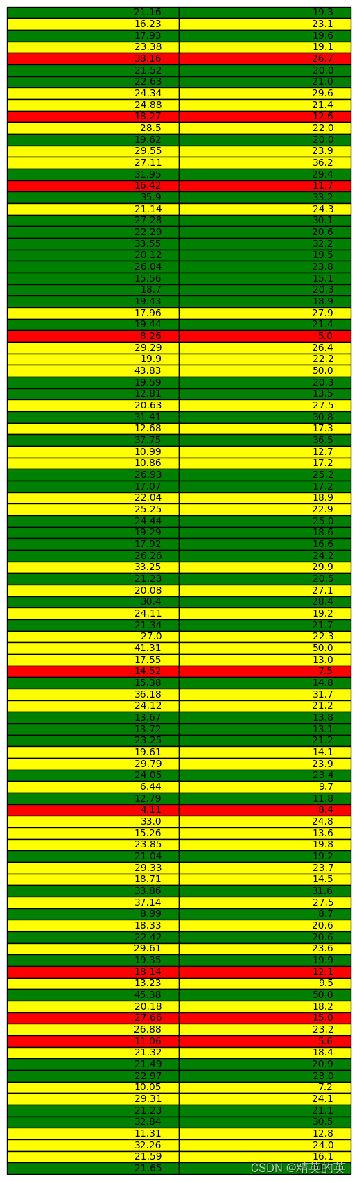
得分展示
完整代码(数据集在绑定资源里,也可以自己去下载)
import numpy as np

def prepare_data(data, normalize_data=True):
    # 标准化特征矩阵(可选)
    if normalize_data:
        features_mean = np.mean(data, axis=0)    #特征的平均值
        features_dev = np.std(data, axis=0)      #特征的标准偏差
        features = (data - features_mean) / features_dev    #标准化数据
    else:
        features_mean = None
        features_dev = None

    # 为特征添加偏置项
    data_processed = np.hstack((np.ones((features.shape[0], 1)), features)).T
    # 返回处理后的数据
    return data_processed, features_mean, features_dev

def get_predict_score(predict_table):
    score_table = []
    pass_count = 0
    for pair in predict_table:
        if (abs(pair[0] - pair[1]) / pair[1] < 0.1):
            score_table.append("good")
            pass_count += 1
        elif (abs(pair[0] - pair[1]) / pair[1] < 0.4):
            score_table.append("around")
            pass_count += 0.8
        else:
            score_table.append("bad")
    accuracy = pass_count / len(predict_table)
    return score_table, accuracy

class LinearRegression:
    '''
    1. 对数据进行预处理操作
    2. 先得到所有的特征个数
    3. 初始化参数矩阵
    '''
    def __init__(self, data,labels, normalize_data = True) -> None:
        (data_proccessed,
         features_mean,
         features_dev) = prepare_data(data, normalize_data)
        self.data = data_proccessed
        self.labels = labels
        self.features_mean = features_mean
        self.features_dev = features_dev
        self.normalize_data = normalize_data

        num_features = self.data.shape[0] #特征个数
        self.theta = np.zeros((num_features,1)) #初始化权重向量

    def train(self, lr, num_iter = 500):
        #训练模块
        cost_history = self.gradient_desent(lr, num_iter) #梯度下降过程
        return self.theta,cost_history

    def gradient_step(self,lr):
        '''
        梯度下降参数更新,使用矩阵运算
        '''
        num_examples = self.data.shape[1] # 多少行
        prediction = LinearRegression.predict(self.data, self.theta) #每次计算所有样本的预测值,使用矩阵乘法
        delta = prediction - self.labels # 偏差向量
        theta = self.theta
        theta -= lr*(1/num_examples)*(np.dot(delta.T, self.data.T)).T #更新权重
        self.theta = theta #记录当前权重参数

    def gradient_desent(self, lr, num_iter):
        cost_history = []
        for _ in range(num_iter): # 在规定的迭代次数里执行训练
            self.gradient_step(lr)
            cost_history.append(self.cost_function(self.data, self.labels)) # 记录损失值,以便可视化展示
        return cost_history

    def cost_function(self,data,labels):
        num_examples = data.shape[0]
        delta = LinearRegression.predict(self.data, self.theta) - labels #偏差
        cost = (1/2)*np.dot(delta.T, delta) #最小二乘法计算损失
        #print(cost.shape)
        return cost[0][0]

    #针对测试集
    def get_cost(self, data, labels):
        data_proccessed = prepare_data(data, self.normalize_data)[0]
        return self.cost_function(data_proccessed, labels)

    def predict_test(self, data):
        data_proccessed = prepare_data(data, self.normalize_data)[0]
        prediction = LinearRegression.predict(data_proccessed, self.theta)
        return prediction
    @staticmethod
    def predict(data, theta):
        prediction = np.dot(data.T, theta) #特征值和权重参数做点积,计算预测值
        return prediction

import pandas as pd
import matplotlib.pyplot as plt
def main():
    data_file = "J:\\MachineLearning\\数据集\\housing.data"
    data = pd.read_csv(data_file, sep="\s+").sample(frac=1).reset_index(drop=True)
    train_data = data.sample(frac=0.8)
    test_data = data.drop(train_data.index)
    input_param_index = 'NOX'
    output_param_index = 'MEDV'
    x_train = train_data[input_param_index].values
    y_train = train_data[output_param_index].values
    x_test = test_data[input_param_index].values
    y_test = test_data[output_param_index].values

    x_train = train_data.iloc[:, :13].values
    y_train = train_data[output_param_index].values.reshape(len(x_train),1)
    x_test = test_data.iloc[:, :13].values
    y_test = test_data[output_param_index].values.reshape(len(test_data),1)
    print(x_train.shape)
    print(y_train.shape)

    linearReg = LinearRegression(x_train, y_train)
    train_theta, loss_history = linearReg.train(0.0001, 50000)
    fomula = 'Y = '
    index = 0
    for w in np.round(train_theta, 2)[1:]:
        fomula += "{}{}X{}".format(" + " if w >=0 else " - " if index != 0 else "", float(abs(w[0])), index)
        index += 1
    fomula += "{}{}".format(" + " if train_theta[0] >= 0 else "-", round(float(abs(train_theta[0][0])), 2))
    print(fomula)
    print(train_theta.shape)
    plt.plot(loss_history)
    plt.show()

    predic_result = np.round(linearReg.predict_test(x_test), 2)
    predict_table = np.column_stack((predic_result, y_test))
    score, accuracy = get_predict_score(predict_table)
    print("Accuracy is {}".format(accuracy))
    color_table = {"good": "green", "around":"yellow", "bad": "red"}
    #print(predic_result)
    fig, ax = plt.subplots()
    table = ax.table(cellText = predict_table, loc = 'center')
    for i, cell in enumerate(table._cells.values()):
        color_index = int(i / 2)
        cell.set_facecolor(color_table[score[color_index]])
    ax.axis("off")
    plt.show()


if (__name__ == "__main__"):
    main()