5. Turing Machine

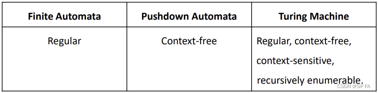
• $k\ge 1$ infinitely long tape (The tape is infinite both to the left and to the right), divided into cells. Each cell stores a symbol belonging to $\Gamma$ (tape alphabet).
• Tape head can move both right and left, one cell per move. It read from or write to a tape.
• State control can be in any one of a finite number of states $Q$. It is based on: state and symbol read from tape.
• Machine has one start state, one accept state and one reject state.
• Machine can run forever: infinite loop.

Properties of Turing Machine

• Turing machine can both read from tape and write on it.
• Tape head can move both right and left.
• Tape is infinite and can be used for storage.
• Accept and reject states take immediate effect.

A Turing machine ™ is a 7-tuple $M=(\Sigma ,\Gamma ,Q,\delta ,q,q_{accept},q_{reject})$, where

• $\Sigma$ is a finite set, called the input alphabet; the blank symbol is not contained in $\Sigma$
• $\Gamma$ is a finite set, called the tape alphabet; this alphabet contains the blank symbol, and $\Sigma \subseteq \Gamma$
• $Q$ is a finite set, whose elements are called states
• $q$ is an element of $Q$; it is called the start state
• $q_{accept}$ is an element of $Q$; it is called the accept state
• $q_{reject}$ is an element of $Q$; it is called the reject state, $q_{reject}\ne q_{accept}$
• $\delta$ is called the transition function, which is a function δ : Q × Γ → Q × Γ × { L , R , N } \delta:Q\timesΓ\rightarrow Q\timesΓ\times\{L,R,N\} δ:Q×Γ→Q×Γ×{L,R,N}
  $L$: move to left, $R$: move to right, $N$: no move.

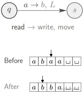
Transition function

$\delta (q,a)=(s,b,L)$

If TM

• in state $q\in Q$
• tape head reads tape symbol $a\in \Gamma$

Then TM

• moves to state $s\in Q$
• overwrites $a$ with $b\in \Gamma$
• moves head left

Computation steps

• Before the computation step, the Turing machine is in a state KaTeX parse error: Undefined control sequence: \inQ at position 2: r\̲i̲n̲Q̲, and the tape head is on a certain cell.
• TM $M$ proceeds according to transition function: δ : Q × Γ → Q × Γ × { L , R , N } \delta:Q\timesΓ\rightarrow Q\timesΓ\times\{L,R,N\} δ:Q×Γ→Q×Γ×{L,R,N}
• Depending on $r$ and $k$ symbols read from tape:
  • switches to a state $r^{\prime }\in Q$
  • tape head writes a symbol of $\Gamma$ in the cell it is currently scanning
  • tape head moves one cell to the left or right or stay at the current cell.
• Computation continues until $q_{reject}$ or $q_{accept}$ is entered.
• Otherwise, $M$ will run forever (input string is neither accepted nor rejected)

Start configuration
The input is a string over the input alphabet $\Sigma$. Initially, this input string is stored on the first tape, and the head of this tape is on the leftmost symbol of the input string.

Computation and termination
Starting in the start configuration, the Turing machine performs a sequence of computation steps. The computation terminates at the moment when the Turing machine enters the accept state $q_{accept}$ or the reject state $q_{reject}$. (If the machine never enters $q_{accept}$ and $q_{reject}$ the computation does not terminate.)

Acceptance
The Turing machine $M$ accepts the input string $w\in {\Sigma }^{\ast }$ , if the computation on this input terminates in the state $q_{accept}$.

5.1 TM Configuration

Configuration of a TM $M=(Q,\Sigma ,\Gamma ,\delta ,q,q_{accept},q_{reject})$ is a string $uqv$ with $u,v\in {\Gamma }^{\ast }$ and $q\in Q$, and specifies that currently

• $M$ is in state $q$
• tape contains $uv$
• tape head is pointing to the cell containing the first symbol in $v$

5.2 TM Transitions

Configuration $C1$ yields configuration $C2$ if the Turing machine can legally go from $C1$ to $C2$ in a single step. For TM $M=(Q,\Sigma ,\Gamma ,\delta ,q,q_{accept},q_{reject})$, suppose

• $u,v\in {\Gamma }^{\ast }$
• $a,b,c\in \Gamma$
• $q_i,q_j\in Q$
• transition function δ : Q × Γ → Q × Γ × { L , R } \delta:Q\timesΓ\rightarrow Q\timesΓ\times\{L,R\} δ:Q×Γ→Q×Γ×{L,R}

5.3 TM Computation

Given a TM $M=(Q,\Sigma ,\Gamma ,\delta ,q,q_{accept},q_{reject})$ and input string $w\in {\Sigma }^{\ast }$. $M$ accepts input $w$ if there is a finite sequence of configurations $C_1,C_2,\dots ,C_k$ for some $k\ge 1$ with

• $C_1$ is the starting configuration $q0w$
• $C_i$ yields $C_{i+1}$ for all $i=1,\dots ,k-1$ ((sequence of configurations obeys transition function $\delta$)
• $C_k$ is an accepting configuration $u{q}_{accept}v$ for some $u,v\in {\Gamma }^{\ast }$

5.4 Language accepted by TM

The language $L(M)$ accepted by the Turing machine $M$ is the set of all strings in ${\Sigma }^{\ast }$ that are accepted by $M$.

Language $A$ is Turing-recognizable if there is a TM $M$ such that $A=L(M)$

• Also called recursively enumerable or enumerable language.
• On an input $w\in L(M)$, the machine $M$ can either halt in a rejecting state, or it can loop indefinitely.
• Turing-recognizable not practical because never know if TM will halt.

5.5 Decider

A decider is TM that halts on all inputs

Language $A=L(M)$ is decided by TM $M$ if on each possible input $w\in {\Sigma }^{\ast }$, the TM finishes in a halting configuration

• $M$ ends in $q_{accept}$ for each $w\in A$
• $M$ ends in $q_{reject}$ for each $w\in A$

$A$ is Turing-decidable if $\exists$ TM $M$ that decides A

• Also called recursive or decidable language.
• Differences to Turing-recognizable language:
  • Turing-decidable language has TM that halts on every string $w\in {\Sigma }^{\ast }$
  • TM for Turing-recognizable language may loop on strings $w\notin$ this language

5.6 Multi-tape TM

• Each tape has its own head
• Transition determined by
  • state
  • the content read by all heads
• Reading and writing of each head are independent of others

A k-tape Turing machine ™ is a 7-tuple $M=(\Sigma ,\Gamma ,Q,\delta ,q,q_{accept},q_{reject})$ has $k$ different tapes and $k$ different read/write heads, where,

• $\Sigma$ is a finite set, called the input alphabet; the blank symbol $ϵ$ is not contained in $\Sigma$.
• $\Gamma$ is a finite set, called the tape alphabet; this alphabet contains the blank symbol $ϵ$, and $\Sigma \subseteq \Gamma$
• $Q$ is a finite set, whose elements are called states
• $q$ is an element of $Q$; it is called the start state
• $q_{accept}$ is an element of $Q$; it is called the accept state
• $q_{reject}$ is an element of $Q$; it is called the reject state
• $\delta$ is called the transition function, which is a function δ : Q × Γ k → Q × Γ k × { L , R , N } k \delta:Q\timesΓ^k\rightarrow Q\timesΓ^k\times\{L,R,N\}^k δ:Q×Γk→Q×Γk×{L,R,N}k
  ${\Gamma }^k=\Gamma \times \Gamma \times \cdots \times \Gamma$

Transition function
δ : Q × Γ k → Q × Γ k × { L , R , N } k \delta:Q\timesΓ^k\rightarrow Q\timesΓ^k\times\{L,R,N\}^k δ:Q×Γk→Q×Γk×{L,R,N}k
Given $\delta (q_i,a_1,a_2,\cdots ,a_k)=(q_j,b_1,b_2,\cdots ,b_k,L,R,\cdots ,L)$

5.6.1 Multi-tape TM equivalent to 1-tape TM

simulate k-tape TM using 1-tape TM

Proof
Let TM $M=(\Sigma ,\Gamma ,Q,\delta ,q,q_{accept},q_{reject})$ be a k-tape TM.

$M$ has:

• input $w=w_1,w_2,\cdots ,w_k$
• other tapes contain only blanks $ϵ$
• each head points to first cell.

Construct 1-tape TM $M^{\prime }$ by extending tape alphabet Γ ′ = Γ ∪ Γ ˙ ∪ { # } Γ^\prime=Γ\cup\dot{Γ}\cup\{\#\} Γ′=Γ∪Γ˙∪{#}where $\dot{\Gamma }$ contains the head positions of different tapes. These positions are marked by dotted symbol.

For each step of k-tape TM $M$, 1-tape $M^{\prime }$ operates its tape as:

• At the start of the simulation, the tape head of $M^{\prime }$ is on the leftmost $\#$
• Scans the tape from first $\#$ to $(k+1)st\#$ to read symbols under heads.
• Rescans to write new symbol and move heads.

Turing recognizable & Multiple-tape TM
Language $L$ is TM-recognizable if and only if some multi-tape TM recognizes $L$.

5.7 Nondeterministic TM

A nondeterministic Turing machine (NTM) M can have several options at every step. It is defined by the 7-tuple $M=(\Sigma ,\Gamma ,Q,\delta ,q,q_{accept},q_{reject})$, where

• $\Sigma$ is input alphabet (withoutblank)
• $\Gamma$ is tape alphabet with { ϵ } ∪ Σ ⊆ Γ \{\epsilon\}\cup\Sigma\subseteqΓ {ϵ}∪Σ⊆Γ
• $Q$ is a finite set, whose elements are called states
• $\delta$ is transition function δ : Q × Γ → P ( Q × Γ × { L , R } ) \delta:Q\timesΓ\rightarrow P(Q\timesΓ\times\{L,R\}) δ:Q×Γ→P(Q×Γ×{L,R})
• $q$ is start state $\in Q$
• $q_{accept}$ is accept state $\in Q$
• $q_{reject}$ is reject state $\in Q$

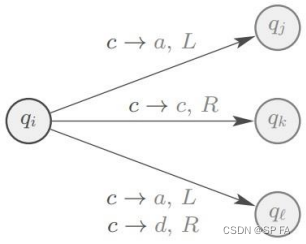
Transition

Computation
With any input $w$, computation of NTM is represented by a configuration tree.

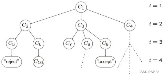
If $\exists$ at least one accepting leaf, then NTM accepts.

5.7.1 Address

Every node in the tree has at most $b$ children. $b$ is size of largest set of possible choices for $N^{\prime }s$ transition function.

• Every node in tree has an address that is a string over the alphabet Γ b = { 1 , 2 , ⋯   , b } Γ_b=\{1,2,\cdots,b\} Γb​={1,2,⋯,b}

5.7.2 NTM equivalent to TM

Every nondeterministic TM has an equivalent deterministic TM.

Proof

• Build TM $D$ to simulate NTM $N$ on each input $w$. $D$ tries all possible branches of $N^{\prime }s$ tree of configurations.
• If $D$ finds any accepting configuration, then it accepts input $w$.
• If all branches reject, then $D$ rejects input $w$.
• If no branch accepts and at least one loops, then $D$ loops on $w$.

1. Initially, input tape contains input string $w$. Simulation and address tapes are initially empty.
2. Copy input tape to simulation tape.
3. Use simulation tape to simulate NTM $N$ on input $w$ on path in tree from root to the address on address tape.
   • At each node, consult next symbol on address tape to determine which branch to take.
   • Accept if accepting configuration reached.
   • Skip to next step if
     • symbols on address tape exhausted.
     • nondeterministic choice invalid
     • rejecting configuration reached
4. Replace string on address tape with next string in ${\Gamma }_b^{\ast }$ in string order, and go to Stage 2.

Turing recognizable & Multiple-tape TM
Language L is TM-recognizable if a NTM recognizes it. Multiple-tape TMs and NTMs are not more powerful than standard TMs.

Turing decidable & NTM decidable
A nondeterministic TM is a decider if all branches halt on all inputs. A language is decidable if some nondeterministic TM decides it.

5.8 Enumerable Language and Enumerator

A language is enumerable if some TM recognizes it.

An enumerator is usually represented as a 2-tape Turing machine. One working tape, and one print tape.

Language A is Turing-recognizable if some enumerator enumerates it.

5.9 Encoding

Input to a Turing machine is a string of symbols over an alphabet

When we want TMs to work on different objects, we need to encode this object as a string of symbols over an alphabet.

5.9.1 Encoding of Graph

Given an undirected graph $G$

$<G>$ of graph $G$ is string of symbols over some alphabet $\Sigma$, where the string starts with list of nodes and followed by list of edges.

5.9.2 TM to decide the connectedness of a Graph

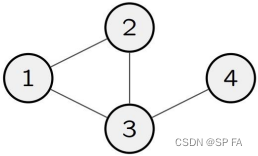
An undirected graph is connected if every node can be reached from any other node by travelling along edge. Let $A$ be the language consisting of strings representing connected undirected graph.

On input $<G>\in \Omega$, where $G$ is an undirected graph

• Check if $G$ is a valid graph encoding. If not, reject.
• Select first node of $G$ and mark it.
• Repeat until no new nodes marked.
• For each node in $G$, mark it if it’s attached by an edge to a node already marked.
• Scan all nodes of $G$ to see whether they all are marked. If they are, accept; otherwise, reject.

$\Omega$ denotes the universe of a decision problem, comprising all instances.

For TM $M$ that decides A = { < G > ∣ G  is a connected undirected graph } A=\{<G>|G\text{ is a connected undirected graph}\} A={<G>∣G is a connected undirected graph} D = { < G > ∣ G  is an undirected graph } D=\{<G>|G\text{ is an undirected graph}\} D={<G>∣G is an undirected graph}

Step 1 checks that input $G\in \Omega$ is valid encoding:

• Two list
  • First is a list of numbers
  • Second is a list of pairs of numbers
• First list contains no duplicate
• Every node in second list appears in first list

Step 2-5 check if $G$ is connected.

---

6. Decidable Languages

6.1 Decidability

Let $\Sigma$ be an alphabet and let $L\subseteq {\Sigma }^{\ast }$ be a language. We say that $L$ is decidable, if there exists a Turing machine $M$, such that for every string $w\in {\Sigma }^{\ast }$, the following holds:

• If $w\in L$, then the computation of the Turing machine $M$, on the input string $w$, terminates in the accept state.
• If $w\notin L$, then the computation of the Turing machine $M$, on the input string $w$, terminates in the reject state.

Given a language $L$ whose elements are pairs of the form $(B,w)$, where

• $B$ is some computation model.
• $w$ is a string over the alphabet $\Sigma$

The pair $(B,w)\in L_B$ iff $w\in L$.

Since the input to computation model $B$ is a string over $\Sigma$, we must encode the pair $(B,w)$ as a string.

6.1.1 The Language $L_{DFA}$ is decidable

Decision problem: Dose a given DFA $B$ accept a given string $w$?
L D F A = { < B , w > ∣ B  is a DFA that accept  w } ⊆ Ω Ω = { < B , w > ∣ B  is a DFA and  w  is a string } \begin{aligned}L_{DFA}&=\{<B,w>|B\text{ is a DFA that accept }w\}\subseteq\Omega\\\Omega&=\{<B,w>|B\text{ is a DFA and }w\text{ is a string}\}\end{aligned} LDFA​Ω​={<B,w>∣B is a DFA that accept w}⊆Ω={<B,w>∣B is a DFA and w is a string}​

To prove $L_{DFA}$ is decidable, we need to construct TM $M$ that decides $L_{DFA}$.

For $M$ that decides $L_{DFA}$:

• take $<B,w>\in \Omega$ as input
• halt and accept if $<B,w>\in L_{DFA}$
• halt and reject if $<B,w>\notin L_{DFA}$

Proof
On input $<B,w>\in \Omega$, where

• $B=(\Sigma ,Q,\delta ,q_0,F)$ is a DFA.
• $w=w_1{w}_2\cdots w_n\in {\Sigma }^{\ast }$ is input string to process on $B$

1. Check if $<B,w>$ is “proper” encoding. If not, reject.
2. Simulate $B$ on $w$ based on:
   • $q\in Q$, the current state of $B$
   • i ∈ { 1 , 2 , ⋯   , ∣ w ∣ } i\in\{1,2,\cdots,|w|\} i∈{1,2,⋯,∣w∣}, the pointer that illustrates the current position in $w$.
   • $q$ changes in accordance with $w_i$ and the transition function $\delta (q,w_i)$.
3. If $B$ ends in $q\in F$, then $M$ accepts; otherwise, reject.

6.1.2 The Language $L_{NFA}$ is decidable

Proof
On input $<B,w>\in \Omega$, where

• $B=(\sigma ,Q,\delta ,q_0,F)$ is a NFA
• $w\in {\Sigma }^{\ast }$ is input string to process on $B$.

1. Check if $<B,w>$ is “proper” encoding. If not, reject.
2. Transform NFA $B$ into DFA $C$.
3. Run TM $M$ for $L_{DFA}$ on input $<C,w>$

6.1.3 The Language $L_{REX}$ is decidable

1. Check if $<R,w>$ is “proper” encoding. If not, reject.
2. Transform regular expression $R$ into DFA $B$.
3. Run TM $M$ for $L_{DFA}$ on input $<C,w>$

6.1.4 CFGs are decidable

1. Check if $<G,w>$ is proper encoding of CFG and string; if not, reject.
2. Convert $G$ into equivalent CFG $G^{\prime }$ in Chomsky normal form.
3. If $w=ϵ$, check if $S\to ϵ$ is a rule of $G^{\prime }$. If so, accept; otherwise, reject.
4. If $w\ne ϵ$, list all derivations with $2n-1$ steps, where $n=|w|$
5. If any generates $w$, accept, otherwise, reject.

6.1.5 CFLs are decidable

1. Let $L$ be a CFL
   • $G^{\prime }$ be a CFG for language $L$.
   • $S$ be a TM that decides A C F G = { < G , w > ∣ G  is a CFG that generates string  w } A_{CFG}=\{<G,w>|G\text{ is a CFG that generates string }w\} ACFG​={<G,w>∣G is a CFG that generates string w}
2. Construct TM $M_{G^{\prime }}$ for language $L$ having CFG $G^{\prime }$ as follows:
   • Run TM decider $S$ on input $<G^{\prime },w>$
   • If $S$ accepts, accept, otherwise, reject.

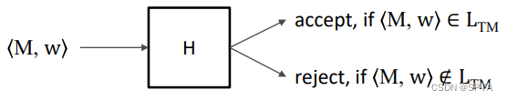
6.1.6 The Language $L_{TM}$ is undecidable

图灵机停机问题是不可判定的，意思即是不存在一个图灵机能够判定任意图灵机对于任意输入是否停机。

1. Suppose $L_{TM}$ is decided by a TM $H$, with input $<M,w>\in \Omega$
   
2. Use $H$ as a subroutine to construct a new TM $D$
   
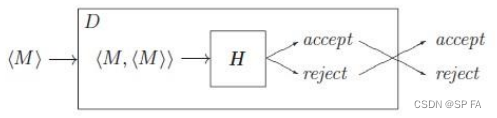
3. If we input the string and take $M=D$
   • If $D$ accept $<D>$, then $D$ rejects $<D>$
   • Clearly a contradiction.

6.2 Unsolvable and Undecidable problems

Undecidable problem. The associated language of a problem cannot be recognized by a TM that halts for all inputs. (one problem that should give a “yes” or “no” answer, but yet no algorithm exists that can answer correctly on all inputs.)

Unsolvable problem. A computational problem that cannot be solved by a TM. Undecidable problem is a subcategory of Unsolvable problem.

6.3 Countable set

Let $A$ and $B$ be two sets. We say that $A$ and $B$ have the same size, if there exists a bijection $f:A\to B$

Let $A$ be a set. We say that $A$ is countable, if $A$ is finite, or $A$ and $N$ have the same size.

Uncountable set

A set is uncountable if it contains so many elements that there is no bijection between this set and the set of natural numbers (N).

---

7. Reducibility

Reduction is a way of converting one problem to another problem, so that the solution to the second problem can be used to solve the first problem.

If $A$ reduces to $B$, then any solution of $B$ solves $A$ (Reduction always involves two problems, $A$ and $B$).

• If $A$ is reducible to $B$, then $A$ cannot be harder than $B$.
• If $A$ is reducible to $B$ and $B$ is decidable, then $A$ is also decidable.
• If $A$ is reducible to $B$ and $A$ is undecidable, then $B$ is also undecidable.

A common strategy for proving that a language $L$ is undecidable is by reduction method, proceeding as follows:
Typical approach to show $L$ is undecidable via reduction from $A$ to $L$:

• Find a problem $A$ known to be undecidable
• Suppose $L$ is decidable.
• Let $R$ be a TM that decides $L$.
• Using $R$ as subroutine to construct another TM $S$ that decides $A$.
• But $A$ is not decidable.
• Conclusion: $L$ is not decidable.

7.1 Computation histories

An accepting computation history for a TM $M$ on a string $w$ is a sequence of configurations $$C_1,C_2,\cdots ,C_k$$ for some $k\ge 1$ such that the following properties hold:

1. $C_1$ is the start configuration of $M$ on $w$.
2. Each $C_j$ yields $C_{j+1}$
3. $C_k$ is an accepting configuration.

A rejecting computation history for $M$ on w is the same except last configuration $C_k$ is a rejecting configuration of $M$.

Accepting and rejecting computation histories are finite.

If $M$ does not halt on $w$, then no accepting or rejecting computation history exists.

Useful for both:

• deterministic TMs (one history).
• nondeterministic TMs (many histories).

$<M,w>\notin A_{TM}$ is equivalent to

• there is no accepting computation history for $M$ on $w$
• all histories are non-accepting ones for $M$ on $w$

7.2 Computable functions

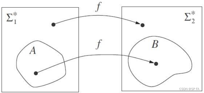
Suppose we have 2 languages $A$ and $B$, where

• $A$ is defined over alphabet ${\Sigma }_1$, so $A\subseteq {\Sigma }_1^{\ast }$
• $B\subseteq {\Sigma }_2^{\ast }$

Informally speaking, $A$ is reducible to $B$ if we can use a black box for $B$ to build an algorithm for $A$.

A function $$f:{\Sigma }_1^{\ast }\to {\Sigma }_2^{\ast }$$ is a computable function if some TM $M$, on every input $w\in {\Sigma }_1^{\ast }$ halts with just $f(w)\in {\Sigma }_2^{\ast }$ on its tape. (there exists a TM can compute this function)
One useful class of computable functions transforms one TM into another.

7.3 Mapping Reducibility

Suppose that $A$ and $B$ are two languages

• $A$ is defined over alphabet ${\Sigma }_1^{\ast }$, so $A\subseteq {\Sigma }_1^{\ast }$
• $B\subseteq {\Sigma }_2^{\ast }$

Then $A$ is mapping reducible to $B$, written$$A{\le }_{m}B$$if there is a computable function$$f:{\Sigma }_1^{\ast }\to {\Sigma }_2^{\ast }$$such that, for every $w\in {\Sigma }_1^{\ast }$$$w\in A\iff f(w)\in B$$The function $f$ is called a reduction of $A$ to $B$

YES instance for problem $A\iff$ YES instance for problem $B$.

Theorem

1. If $A{\le }_{m}B$ and $B$ is decidable, then $A$ is decidable.
2. If $A{\le }_{m}B$ and $B$ is Turing-recognizable, then $A$ is Turing-recognizable.

Corollary
3. If $A{\le }_{m}B$ and $A$ is undecidable, then $B$ is undecidable.
4. If $A{\le }_{m}B$ and $A$ is not Turing-recognizable, then $B$ is not Turing-recognizable.

7.4 Algorithm and Information

Algorithm is independent of computation model

All reasonable variants of TM models are equivalent to TM:

• k-tape TM
• nondeterministic TM
• enumerator
• random-access TM: head can jump to any cell in one step

Similarly, all “reasonable” programming languages are equivalent. The notion of an algorithm is independent of the computation model.

7.4.1 Algorithm

Informally

• a recipe
• a procedure
• a computer program

Historically

• algorithms have long history in mathematics
• but not precisely defined until 20th century
• informal notions rarely questioned, but insufficient to show a problem has no algorithm.

7.4.2 Information

We define the quantity of information contained in an object to be the size of that object’s smallest representation or description (a precise and
unambiguous characterization of the object so that we may recreate it from the description alone.).

Minimal length description
Many types of description language can be used to define information. Selecting which language to use affects the characteristics of the definition.

In this class, our description languages is based on algorithms.

One way to use algorithms to describe strings is to construct a Turing machine that prints out the string when it is started on a blank tape and then represent that Turing machine itself as a string.

Drawback to this approach:
A Turing machine cannot represent a table of information concisely with its transition function. To represent a string of $n$ bits, you might use $n$ states and $n$ rows in the transition function table. That would result in a description that is excessively long for our purpose.

We describe a binary string $x$ with a Turing machine $M$ and a binary input $w$ to $M$. The length of the description is the combined length of representing $M$ and $w$.

• Writing this description with our usual notation for encoding several objects into a single binary string $<M,w>$.
• To produce a concise result, we define the string $<M,w>$ to be $<M>w$

However, we might run into trouble if directly concatenating $w$ onto the end of $M$. The point at which $<M>$ ends and $w$ begins is not discernible from the description itself. We avoid this problem by ensuring that we can locate the separation between $<M>$ and $w$ in $<M>w$.

Let $x$ be a binary string. The minimal description of $x$, written $d(x)$, is the shortest string $<M,w>$ where TM $M$ on input $w$ halts with $x$ on its tape. The descriptive complexity of $x$, written $K(x)$, is$$K(x)=|d(x)|$$

• The definition of K(x) is intended to capture our intuition for the amount of information in the string x.

Theorem 1
$$\exists c\forall x[K(x)\le |x|+c]$$

This theorem says that the descriptive complexity of a string is at most a fixed constant more than its length. The constant is a universal one, not dependent on the string.

Theorem 2
$$\exists c\forall x,y[K(xy)\le 2K(x)+K(y)+c]$$

The cost of combining two descriptions leads to a bound that is greater than the sum of the individual complexities.

7.5 Recursively Enumerable Languages

7.5.1 Enumerability

Let $\Sigma$ be an alphabet and let $L\subseteq {\Sigma }^{\ast }$ be a language. We say that $L$ is enumerable, if
there exists a Turing machine $M$, such that for every string $w\in {\Sigma }^{\ast }$, the following holds:

1. if $w\in A$, then the computation of the $M$, on the input string $w$, terminates in the accept state.
2. if $w\notin A$, then either the computation terminates in the reject state or the computation does not terminate.

From the perspective of algorithm
The language $L$ is enumerable, if there exists an algorithm having the following property:

1. if $w\in A$, then the algorithm terminates on the input string $w$ and tells us that $w\in A$
2. if $w\notin A$, then either
   • the algorithm terminates on the input string $w$ and tells us that $w\notin A$
   • the algorithm does not terminate on the input string $w$, in which case it does not tell us that $w\notin A$

7.5.2 Recursively Enumerable Languages

A language $L$ is recursively enumerable if there exists a TM $M$ such that $L=L(M)$.
A language $L$ over $\Sigma$ is recursive if there exists a TM $M$ such that $L=L(M)$ and $M$ halts on every $w\in {\Sigma }^{\ast }$

There is only a slight difference between recursively enumerable and recursive languages. In the first case we do not require the Turing machine to terminate on every input word.

递归语言、递归可枚举语言和非递归可枚举语言

Enumeration procedure for recursive languages
To enumerate all $w\in {\Sigma }^{\ast }$ in a recursive language $L$:

• Let $M$ be a TM that recognizes $L$, $L=L(M)$
• Construct 2-tape TM $M^{\prime }$: Tape 1 will enumerate the strings in ${\Sigma }^{\ast }$, tape 2 will enumerate the strings in $L$.
  • On tape 1 generate the next string $v\in {\Sigma }^{\ast }$
  • Simulate $M$ on $v$ (if $M$ accepts $v$, then write $v$ on tape 2).

Enumeration procedure for r.e languages
To enumerate all $w\in {\Sigma }^{\ast }$ in a recursively enumerable language $L$:

Repeat

• Generate next string (Suppose k strings have been generated: $w_1,w_2,\cdots ,w_k$)
• Run $M$ for one step on $w_k$, run $M$ for two steps on $w_{k-1}$… Run $M$ for $k$ steps on $w_1$. If any of the strings are accepted then write them to tape 2.

7.5.3 Decidability and Undecidability

“Decidable” is a synonym for “recursive.” We tend to refer to languages as “recursive” and problems as “decidable”.

If a language is not recursive, then we call the problem expressed by that language “undecidable”.

Theorem
Every decidable language is enumerable. (Converse is not correct)

7.5.4 The Language $L_{TM}$

The language L T M = { < M , w > : M  is a Turing machine that accepts the string w } L_{TM}=\{<M,w>:M\text{ is a Turing machine that accepts the string} w\} LTM​={<M,w>:M is a Turing machine that accepts the stringw} is undecidable

Theorem
The language $L_{TM}$ is enumerable

7.5.5 Enumerator

Let $\Sigma$ be an alphabet and let $L\subset {\Sigma }^{\ast }$ be a language. An enumerator for $L$ is a Turing machine $M$ having the following properties:

1. $M$ has a print tape and a print state. During its computation, $M$ writes symbols of $\Sigma$ on the print tape. Each time, $M$ enters the print state, the current string on the print tape is sent to the printer and the print tape is made empty.
2. At the start of the computation, all tapes are empty and $M$ is in the start state.
3. Every string $w$ in $L$ is sent to the printer at least once.
4. Every string $w$ that is not in $L$ is never sent to the printer.

Theorem
A language is enumerable if and only if it has an enumerator.

7.6 Complexity Theory

If we can solve a problem $P$, how easy or hard is it to do so?

Counting Resources
We have two ways to measure the “hardness” of a problem:

• Time Complexity: how many time-steps are required in the computation of a problem?
• Space Complexity: how many bits of memory are required for the computation?

7.6.1 Running time

Let $M$ be a Turing machine, and let $w$ be an input string for $M$. We define the running time $f(|w|)$ of $M$ on input $w$ as the number of computation steps made by $M$ on input $w$.
As usual, we denote by $|w|$, the number of symbols in the string $w$.

• The exact running time of most algorithms is complex.
• To large problems, try to use an approximation instead.
• Sometimes, only focus on the “important ” part of running time.

Let $\Sigma$ be an alphabet, let $T:N_0\to N_0$ be a function, let $A\subseteq {\Sigma }^{\ast }$ be a decidable language, and let $F:{\Sigma }^{\ast }\to {\Sigma }^{\ast }$ be a computable function.
We say that the Turing machine $M$ decides the language $A$ in time $T$, if$$f(|w|)\le T(|w|)$$for all strings $w$ in ${\Sigma }^{\ast }$.
We say that the Turing machine $M$ computes the function $F$ in time $T$, if$$f(|w|)\le T(|w|)$$for all strings $w$ in ${\Sigma }^{\ast }$

7.6.2 Asymptotic Notation

We typically measure the computational efficiency as the number of a basic operations it performs as a function of its input length.

The computation efficiency can be captured by a function $T$ from the set of natural numbers $N$ to itself such that $T(n)$ is equal to the maximum number of basic operations that the algorithm performs on inputs of length $n$.

However, this function is sometimes be overly dependent on the low-level
details of our definition of a basic operation.

Big-O Notation
Given functions $f$ and $g$, where$$f,g:N\to R^{+}$$We say that$$f(n)=O(g(n))$$if there are two positive constants $c$ and $n_0$ such that$$f(n)\le c\cdot g(n)\text{ for all }n\ge n_0$$where $n=|w|$

We say that $g(n)$ is an asymptotic upper bound on $f(n)$

Polynomials
$$p(n)=a_1{n}^{k_1}+a_2{n}^{k_2}+\cdots +a_d{n}^{k_d}$$where $k_1>k_2>\cdots >k_d\ge 0$, then

• $p(n)=O(n^{k_1})$
• Also, $p(n)=O(n^r)$ for all $r\ge k_1$

Exponential
Exponential functions like $2^n$ always eventually “overpower” polynomials.

• For all constants $a$ and $k$, polynomial $f(n)=a\cdot n^k+\cdots$ obeys:$$f(n)=O(2^n)$$
• For functions in $n$, we have$$n^k=O(b^n)$$for all positive constants $k$ and $b>1$

Logarithms
$$f(n)=O(\log n)$$

Little-o Notation
Given two functions $f$ and $g$, where$$f,g:N\to R^{+}$$We say that$$f(n)=o(g(n))$$if$$\underset{n\to \infty }{\lim }\frac{f(n)}{g(n)}=0$$

Big-O notation is about “asymptotically less than or equal to”. Little-o is about “asymptotically much smaller than”.