二维离散傅里叶变换的实现
- 1.使用Python包实现
- 2.使用c++实现
- 2.1 FFTW库安装
- 2.2 结果比较
- 参考文献
1.使用Python包实现
import numpy as np
import matplotlib.pyplot as plt
a=np.array([0, 2, 4, 1,6, 1, 3, 2,5]).reshape(3,3)
f=np.fft.fft2(a)
fshift=np.fft.fftshift(f)
mag=20*np.log(np.abs(fshift))
plt.axis("off")
plt.imshow(mag)
plt.show()
其中:
f:
array([[24. +0.00000000e+00j, -6. +4.44089210e-16j, -6. -4.44089210e-16j],
       [-3. +1.73205081e+00j, -7.5+4.33012702e+00j,  4.5-8.66025404e-01j],
       [-3. -1.73205081e+00j,  4.5+8.66025404e-01j, -7.5-4.33012702e+00j]])

fshift:
array([[-7.5-4.33012702e+00j, -3. -1.73205081e+00j,  4.5+8.66025404e-01j],
       [-6. -4.44089210e-16j, 24. +0.00000000e+00j, -6. +4.44089210e-16j],
       [ 4.5-8.66025404e-01j, -3. +1.73205081e+00j, -7.5+4.33012702e+00j]])
平移后的幅度谱为:

2.使用c++实现
#include <iostream>
using namespace std;
#include"Eigen/Dense"
using namespace Eigen;
#include "fftw3.h"

int main()
{

	MatrixXd a(3, 3), out(a.rows(), a.cols());
	MatrixXcd FTa(a.rows() / 2 + 1, a.cols());
	a << 0, 2, 4, 1,
		6, 1, 3, 2,5;
	fftw_plan P;
	P = fftw_plan_dft_r2c_2d(a.cols(), a.rows(), a.data(), (fftw_complex*)FTa.data(), FFTW_ESTIMATE);
	fftw_execute(P);
	cout << "dft" << endl;

	cout << FTa << endl;
	cout << endl;

	P = fftw_plan_dft_c2r_2d(a.cols(), a.rows(), (fftw_complex*)FTa.data(), out.data(), FFTW_ESTIMATE);
	fftw_execute(P);
	cout << "idft" << endl;

	out = out / (a.cols() * a.rows());
	cout << out << endl;
	return 0;
}
结果如下:
dft
         (24,0)          (-6,0)          (-6,0)
   (-3,1.73205)  (-7.5,4.33013) (4.5,-0.866025)

idft
0 2 4
1 6 1
3 2 5
2.1 FFTW库安装
这里用到了FFTW c++库,具体编译及调用可参考Windows下FFTW_2.1.5的编译及使用。
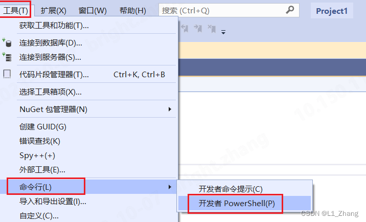
这里仅列出生成lib文件,用到的vs中powetshell打开方式:
2.2 结果比较
从结果可以看出,与Python代码相比,FFTW的输出未进行shift,而且仅输出部分有用信息。
参考文献
[1] FFTW库官网
[2] Windows下FFTW_2.1.5的编译及使用