目录
一、实验介绍
二、实验环境
1. 配置虚拟环境
2. 库版本介绍
3. IDE
三、实验内容
0. 导入必要的工具
1. cal_pearson(计算皮尔逊相关系数)
2. 主程序
a. 实验1(较强的正相关关系):
b. 实验2(几乎没有线性相关关系):
c. 实验3(非常强的正相关关系):
d. 实验4(斯皮尔曼相关系数矩阵):
3. 代码整合
一、实验介绍
本实验主要实现了自定义皮尔逊相关系数进行相关性分析。
相关性分析是一种常用的统计方法,用于评估两个或多个变量之间的关联程度。在本实验中,我们使用了皮尔逊相关系数和斯皮尔曼相关系数这两种常见的相关性指标。皮尔逊相关系数用于度量两个连续变量之间的线性关系,而斯皮尔曼相关系数则适用于评估两个变量之间的任何单调关系,无论是否线性。
二、实验环境
本系列实验使用了PyTorch深度学习框架,相关操作如下(基于深度学习系列文章的环境):
1. 配置虚拟环境
深度学习系列文章的环境
conda create -n DL python=3.7 conda activate DLpip install torch==1.8.1+cu102 torchvision==0.9.1+cu102 torchaudio==0.8.1 -f https://download.pytorch.org/whl/torch_stable.html
conda install matplotlibconda install scikit-learn新增加
conda install pandasconda install seabornconda install networkxconda install statsmodelspip install pyHSICLasso注:本人的实验环境按照上述顺序安装各种库,若想尝试一起安装(天知道会不会出问题)
2. 库版本介绍
| 软件包 | 本实验版本 | 目前最新版 |
| matplotlib | 3.5.3 | 3.8.0 |
| numpy | 1.21.6 | 1.26.0 |
| python | 3.7.16 | |
| scikit-learn | 0.22.1 | 1.3.0 |
| torch | 1.8.1+cu102 | 2.0.1 |
| torchaudio | 0.8.1 | 2.0.2 |
| torchvision | 0.9.1+cu102 | 0.15.2 |
新增
| networkx | 2.6.3 | 3.1 |
| pandas | 1.2.3 | 2.1.1 |
| pyHSICLasso | 1.4.2 | 1.4.2 |
| seaborn | 0.12.2 | 0.13.0 |
| statsmodels | 0.13.5 | 0.14.0 |
3. IDE
建议使用Pycharm(其中,pyHSICLasso库在VScode出错,尚未找到解决办法……)
win11 安装 Anaconda(2022.10)+pycharm(2022.3/2023.1.4)+配置虚拟环境_QomolangmaH的博客-CSDN博客https://blog.csdn.net/m0_63834988/article/details/128693741https://blog.csdn.net/m0_63834988/article/details/128693741![]() https://blog.csdn.net/m0_63834988/article/details/128693741
https://blog.csdn.net/m0_63834988/article/details/128693741
三、实验内容
0. 导入必要的工具
import numpy as np
from scipy import stats
import matplotlib.pyplot as plt
1. cal_pearson(计算皮尔逊相关系数)
def cal_pearson(x, y):
    n = len(x)

    mean_x = np.mean(x)
    mean_y = np.mean(y)

    x_ = x - mean_x
    y_ = y - mean_y

    s_x = np.sqrt(np.sum(x_ * x_))
    s_y = np.sqrt(np.sum(y_ * y_))

    r = np.sum((x_ / s_x) * (y_ / s_y))
    t = r / np.sqrt((1 - r * r) / (n - 2))  # p值需要对t值进行查表获得

    return r
-
计算变量 x 的长度,即样本个数。
-
计算变量 x 、 y 的均值。
-
计算变量 x、 y 的标准差。
-
计算皮尔逊相关系数 r,即将 x_ 和 y_ 中对应位置的值相除,然后相乘后求和。
-
计算 t 值,即将 r 的值除以 sqrt((1 - r^2) / (n - 2))。这里的 n - 2 是修正因子,用于校正样本量对 t 值的影响。
-
返回计算得到的皮尔逊相关系数 r。
2. 主程序
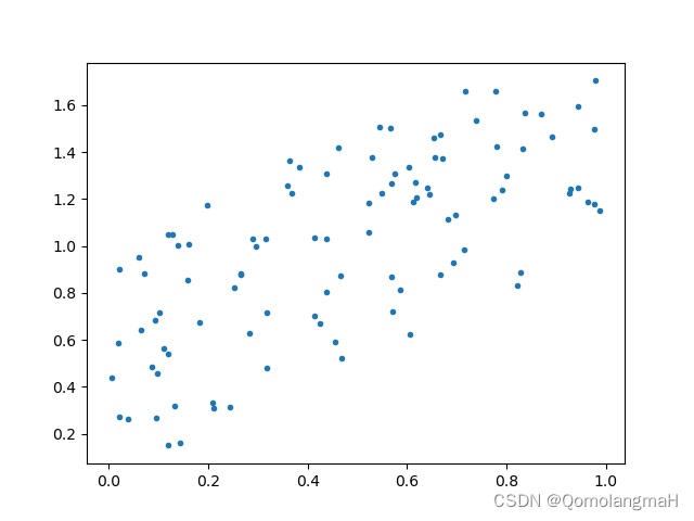
a. 实验1(较强的正相关关系):
    x1 = np.random.random(100)
    y1 = np.random.random(100) + x1
    plt.scatter(x1, y1, marker='.')
    plt.show()
    pearson1, p1 = stats.pearsonr(x1, y1)
    r1 = cal_pearson(x1, y1)
    print(pearson1)
    print(r1)
print()- 生成两个长度为100的随机数组x1和y1,其中y1是在x1的基础上加上一些随机噪声。
- 绘制x1和y1的散点图。
- 使用
scipy.stats.pearsonr函数计算了x1和y1的皮尔逊相关系数和p值, - 使用自定义的
cal_pearson函数计算了相同的相关系数。
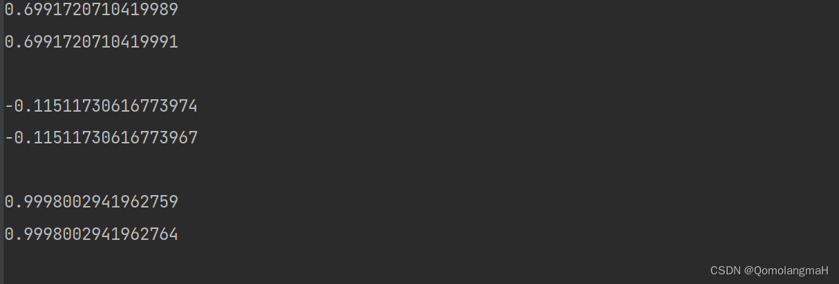
0.6991720710419989
0.6991720710419991
b. 实验2(几乎没有线性相关关系):
    x2 = np.random.random(100)
    y2 = np.random.random(100)
    plt.scatter(x2, y2, marker='.')
    plt.show()
    pearson2, p2 = stats.pearsonr(x2, y2)
    r2 = cal_pearson(x2, y2)
    print(pearson2)
    print(r2)
    print()
生成了两个长度为100的随机数组x2和y2,没有加入噪声。同样绘制了散点图,并分别计算了皮尔逊相关系数。
-0.11511730616773974
-0.11511730616773967
c. 实验3(非常强的正相关关系):
生成了两个长度为100的随机数组x3和y3,其中y3是在x3的基础上加上一些较大的随机噪声。同样绘制了散点图,并分别计算了皮尔逊相关系数。
    x3 = np.random.random(100)
    y3 = np.random.random(100) + x3 * 50
    plt.scatter(x3, y3, marker='.')
    plt.show()
    pearson3, p3 = stats.pearsonr(x3, y3)
    r3 = cal_pearson(x3, y3)
    print(pearson3)
    print(r3)
    print()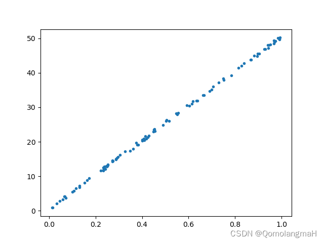
d. 实验4(斯皮尔曼相关系数矩阵):
生成了一个形状为(10, 10)的随机数组data,使用scipy.stats.spearmanr函数计算了data中各列之间的斯皮尔曼相关系数和p值,并将结果打印输出。
    data = np.random.random((10, 10))
    spearman_np, p_np = stats.spearmanr(data)
    print(spearman_np, p_np)
3. 代码整合
import numpy as np
from scipy import stats
import matplotlib.pyplot as plt


def cal_pearson(x, y):
    n = len(x)

    mean_x = np.mean(x)
    mean_y = np.mean(y)

    x_ = x - mean_x
    y_ = y - mean_y

    s_x = np.sqrt(np.sum(x_ * x_))
    s_y = np.sqrt(np.sum(y_ * y_))

    r = np.sum((x_ / s_x) * (y_ / s_y))
    t = r / np.sqrt((1 - r * r) / (n - 2))  # p值需要对t值进行查表获得

    return r


if __name__ == '__main__':
    np.random.seed(0)

    x1 = np.random.random(100)
    y1 = np.random.random(100) + x1
    plt.scatter(x1, y1, marker='.')
    plt.show()
    pearson1, p1 = stats.pearsonr(x1, y1)
    r1 = cal_pearson(x1, y1)
    print(pearson1)
    print(r1)
    print()

    x2 = np.random.random(100)
    y2 = np.random.random(100)
    plt.scatter(x2, y2, marker='.')
    plt.show()
    pearson2, p2 = stats.pearsonr(x2, y2)
    r2 = cal_pearson(x2, y2)
    print(pearson2)
    print(r2)
    print()

    x3 = np.random.random(100)
    y3 = np.random.random(100) + x3 * 50
    plt.scatter(x3, y3, marker='.')
    plt.show()
    pearson3, p3 = stats.pearsonr(x3, y3)
    r3 = cal_pearson(x3, y3)
    print(pearson3)
    print(r3)
    print()

    data = np.random.random((10, 10))
    spearman_np, p_np = stats.spearmanr(data)
    print(spearman_np, p_np)