目录
一:Kaggle数据集准备
二:数据集分析
三:空值处理
四:空值填充
五:查找所有字符列
六:实例化独热编码对象
七:方差过滤
八:特征数据提取
九:查看特征之间的相关系数
十:皮尔逊系数重排
十一:热力图绘制
十二:数据集划分
十三:网格模型 超参调优
十四:训练模型 预测实际比对
十五:完整源码分享
一:Kaggle数据集准备
Kaggle官网下载


二:数据集分析
2-1 表头数据分析
table_head = "Id,MSSubClass,MSZoning,LotFrontage,LotArea,Street,Alley,LotShape,LandContour,Utilities,LotConfig,LandSlope,Neighborhood,Condition1,Condition2,BldgType,HouseStyle,OverallQual,OverallCond,YearBuilt,YearRemodAdd,RoofStyle,RoofMatl,Exterior1st,Exterior2nd,MasVnrType,MasVnrArea,ExterQual,ExterCond,Foundation,BsmtQual,BsmtCond,BsmtExposure,BsmtFinType1,BsmtFinSF1,BsmtFinType2,BsmtFinSF2,BsmtUnfSF,TotalBsmtSF,Heating,HeatingQC,CentralAir,Electrical,1stFlrSF,2ndFlrSF,LowQualFinSF,GrLivArea,BsmtFullBath,BsmtHalfBath,FullBath,HalfBath,BedroomAbvGr,KitchenAbvGr,KitchenQual,TotRmsAbvGrd,Functional,Fireplaces,FireplaceQu,GarageType,GarageYrBlt,GarageFinish,GarageCars,GarageArea,GarageQual,GarageCond,PavedDrive,WoodDeckSF,OpenPorchSF,EnclosedPorch,3SsnPorch,ScreenPorch,PoolArea,PoolQC,Fence,MiscFeature,MiscVal,MoSold,YrSold,SaleType,SaleCondition,SalePrice"
head_list = table_head.split(',')
print(head_list, len(head_list))
['Id', 'MSSubClass', 'MSZoning', 'LotFrontage', 'LotArea', 'Street', 'Alley', 'LotShape', 'LandContour', 'Utilities', 'LotConfig', 'LandSlope', 'Neighborhood', 'Condition1', 'Condition2', 'BldgType', 'HouseStyle', 'OverallQual', 'OverallCond', 'YearBuilt', 'YearRemodAdd', 'RoofStyle', 'RoofMatl', 'Exterior1st', 'Exterior2nd', 'MasVnrType', 'MasVnrArea', 'ExterQual', 'ExterCond', 'Foundation', 'BsmtQual', 'BsmtCond', 'BsmtExposure', 'BsmtFinType1', 'BsmtFinSF1', 'BsmtFinType2', 'BsmtFinSF2', 'BsmtUnfSF', 'TotalBsmtSF', 'Heating', 'HeatingQC', 'CentralAir', 'Electrical', '1stFlrSF', '2ndFlrSF', 'LowQualFinSF', 'GrLivArea', 'BsmtFullBath', 'BsmtHalfBath', 'FullBath', 'HalfBath', 'BedroomAbvGr', 'KitchenAbvGr', 'KitchenQual', 'TotRmsAbvGrd', 'Functional', 'Fireplaces', 'FireplaceQu', 'GarageType', 'GarageYrBlt', 'GarageFinish', 'GarageCars', 'GarageArea', 'GarageQual', 'GarageCond', 'PavedDrive', 'WoodDeckSF', 'OpenPorchSF', 'EnclosedPorch', '3SsnPorch', 'ScreenPorch', 'PoolArea', 'PoolQC', 'Fence', 'MiscFeature', 'MiscVal', 'MoSold', 'YrSold', 'SaleType', 'SaleCondition', 'SalePrice'] 81得出,feature特征有 80列,label标签 有1列
2-2 数据集加载,读取csv
import pandas as pd
import numpy as np

data_df = pd.read_csv("train.csv", sep=',')
print(data_df.head(), data_df.shape)
   Id  MSSubClass MSZoning  ...  SaleType  SaleCondition SalePrice
0   1          60       RL  ...        WD         Normal    208500
1   2          20       RL  ...        WD         Normal    181500
2   3          60       RL  ...        WD         Normal    223500
3   4          70       RL  ...        WD        Abnorml    140000
4   5          60       RL  ...        WD         Normal    250000

[5 rows x 81 columns] (1460, 81)
2-2-1 可以设置显示所有列
# 设置显示所有行、列
pd.set_option("display.max_columns", None)
2-2-2 设置显示所有行
# 设置显示所有行、列
pd.set_option("display.max_rows", None)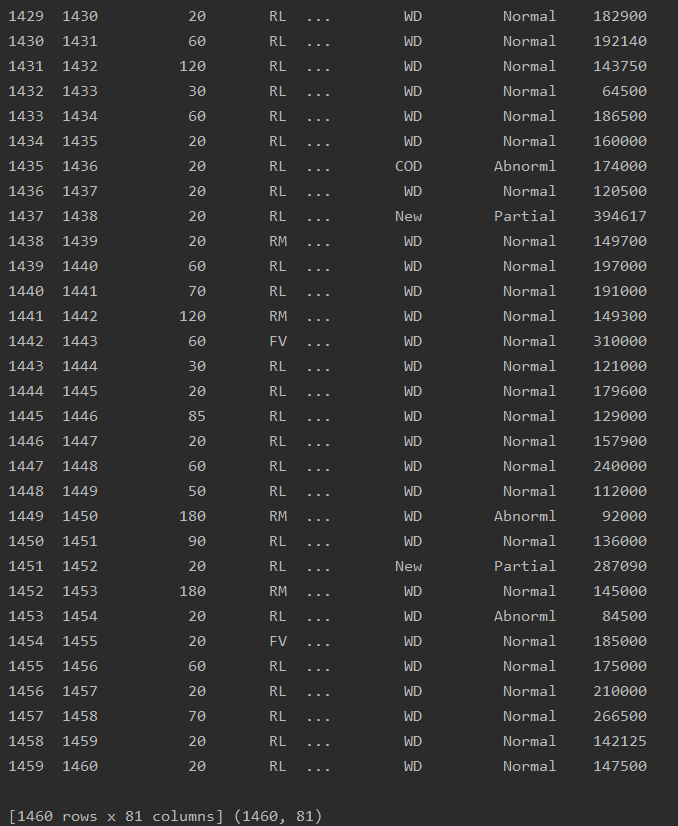
1460*80 即1460行80列 (只看特征数据,不看标签数据)
三:空值处理
空值处理 超过1/3列的直接剔除
# 空值处理
# print(data_df.isnull().sum())
# 超过1/3列的剔除
data_df.drop(columns=['Alley', 'FireplaceQu', 'PoolQC', 'Fence', 'MiscFeature'],
             axis=1, inplace=True)
print(data_df.shape)
LotFrontage 259
Alley 1369 --剔除
MasVnrType 8
BsmtQual 37
BsmtCond 37
BsmtExposure 38
BsmtFinType1 37
BsmtFinType2 38
Electrical 1
FireplaceQu 690 --剔除
GarageType 81
GarageYrBlt 81
GarageFinish 81
GarageQual 81
GarageCond 81
PoolQC 1453 --剔除
Fence 1179 --剔除
MiscFeature 1406 --剔除feature +label
特征数据+标签数据
结果如下
(1460, 76)只计算feature特征数据则为
(1460, 75)四:空值填充
空值填充的填充方式,分为两种,数字列与字符列分别处理,处理方式为:
数字列 [均值、众数、中位数]
字符列 [众数]
首先,可以通过打印出每一列,找出数字列和字符列,结果如下
LotFrontage       259    --数字列
Alley            1369  --剔除
MasVnrType          8  --字符列
MasVnrArea          8    --数字列
BsmtQual           37  --字符列
BsmtCond           37  --字符列
BsmtExposure       38  --字符列
BsmtFinType1       37  --字符列
BsmtFinType2       38  --字符列
Electrical          1  --字符列
FireplaceQu       690  --剔除
GarageType         81  --字符列
GarageYrBlt        81    --数字列
GarageFinish       81  --字符列
GarageQual         81  --字符列
GarageCond         81  --字符列
PoolQC           1453  --剔除
Fence            1179  --剔除
MiscFeature      1406  --剔除
4-1 数字列填充
# 2 空值填充
# 2-1 [数字列]填充
data_df['LotFrontage'].fillna(data_df['LotFrontage'].mean(), inplace=True)
data_df['GarageYrBlt'].fillna(data_df['GarageYrBlt'].median(), inplace=True)
data_df['MasVnrArea'].fillna(data_df['MasVnrArea'].median(), inplace=True)
print(data_df.isnull().sum())
结果如下,LotFrontage、GarageYrBlt、MasVnrArea三个数字列,填充完成
Id                0
MSSubClass        0
MSZoning          0
LotFrontage       0
LotArea           0
Street            0
LotShape          0
LandContour       0
Utilities         0
LotConfig         0
LandSlope         0
Neighborhood      0
Condition1        0
Condition2        0
BldgType          0
HouseStyle        0
OverallQual       0
OverallCond       0
YearBuilt         0
YearRemodAdd      0
RoofStyle         0
RoofMatl          0
Exterior1st       0
Exterior2nd       0
MasVnrType        8
MasVnrArea        0
ExterQual         0
ExterCond         0
Foundation        0
BsmtQual         37
BsmtCond         37
BsmtExposure     38
BsmtFinType1     37
BsmtFinSF1        0
BsmtFinType2     38
BsmtFinSF2        0
BsmtUnfSF         0
TotalBsmtSF       0
Heating           0
HeatingQC         0
CentralAir        0
Electrical        1
1stFlrSF          0
2ndFlrSF          0
LowQualFinSF      0
GrLivArea         0
BsmtFullBath      0
BsmtHalfBath      0
FullBath          0
HalfBath          0
BedroomAbvGr      0
KitchenAbvGr      0
KitchenQual       0
TotRmsAbvGrd      0
Functional        0
Fireplaces        0
GarageType       81
GarageYrBlt       0
GarageFinish     81
GarageCars        0
GarageArea        0
GarageQual       81
GarageCond       81
PavedDrive        0
WoodDeckSF        0
OpenPorchSF       0
EnclosedPorch     0
3SsnPorch         0
ScreenPorch       0
PoolArea          0
MiscVal           0
MoSold            0
YrSold            0
SaleType          0
SaleCondition     0
SalePrice         0
dtype: int64
4-2 字符列处理
4-2-1 获取缺失列名字
# 2-2 剩余的[字符列]在miss_col_list中
# 获取缺失列的名字
miss_col_list = data_df.isnull().any()[data_df.isnull().any().values == True].index.tolist()
# print(data_df.isnull().any())
print(miss_col_list)
['MasVnrType', 'BsmtQual', 'BsmtCond', 'BsmtExposure', 'BsmtFinType1', 'BsmtFinType2', 'Electrical', 'GarageType', 'GarageFinish', 'GarageQual', 'GarageCond']4-2-2 获取缺失列对应的列值
获取缺失列对应的列值 :单个查看
查看不出什么,需要查看全部信息才便于分析数据
# 获取缺失列对应的列值--list
for i in miss_col_list:
    print(data_df[i].values.reshape(-1, 1))
    break
[['BrkFace']
['None']
['BrkFace']
...
['None']
['None']
['None']]获取缺失列对应的列值 :全部查看
接下来众数填充
# 获取缺失列对应的列值--list
miss_list = []

for i in miss_col_list:
    miss_list.append(data_df[i].values.reshape(-1, 1))  # 任意行 列数为1
print(miss_list)
这样查看缺失值对应的列值,思路就比较清晰
[array([['BrkFace'],
       ['None'],
       ['BrkFace'],
       ...,
       ['None'],
       ['None'],
       ['None']], dtype=object), array([['Gd'],
       ['Gd'],
       ['Gd'],
       ...,
       ['TA'],
       ['TA'],
       ['TA']], dtype=object), array([['TA'],
       ['TA'],
       ['TA'],
       ...,
       ['Gd'],
       ['TA'],
       ['TA']], dtype=object), array([['No'],
       ['Gd'],
       ['Mn'],
       ...,
       ['No'],
       ['Mn'],
       ['No']], dtype=object), array([['GLQ'],
       ['ALQ'],
       ['GLQ'],
       ...,
       ['GLQ'],
       ['GLQ'],
       ['BLQ']], dtype=object), array([['Unf'],
       ['Unf'],
       ['Unf'],
       ...,
       ['Unf'],
       ['Rec'],
       ['LwQ']], dtype=object), array([['SBrkr'],
       ['SBrkr'],
       ['SBrkr'],
       ...,
       ['SBrkr'],
       ['FuseA'],
       ['SBrkr']], dtype=object), array([['Attchd'],
       ['Attchd'],
       ['Attchd'],
       ...,
       ['Attchd'],
       ['Attchd'],
       ['Attchd']], dtype=object), array([['RFn'],
       ['RFn'],
       ['RFn'],
       ...,
       ['RFn'],
       ['Unf'],
       ['Fin']], dtype=object), array([['TA'],
       ['TA'],
       ['TA'],
       ...,
       ['TA'],
       ['TA'],
       ['TA']], dtype=object), array([['TA'],
       ['TA'],
       ['TA'],
       ...,
       ['TA'],
       ['TA'],
       ['TA']], dtype=object)]
4-2-3 对每一列进行众数填充
# 对每一列进行众数填充
for i in range(0, len(miss_list)):
    im_most = SimpleImputer(strategy='most_frequent')
    most = im_most.fit_transform(miss_list[i])
    data_df.loc[:, miss_col_list[i]] = most

print(data_df.isnull().sum())
填充完毕,检查输出结果 ,没有问题
Id               0
MSSubClass       0
MSZoning         0
LotFrontage      0
LotArea          0
Street           0
LotShape         0
LandContour      0
Utilities        0
LotConfig        0
LandSlope        0
Neighborhood     0
Condition1       0
Condition2       0
BldgType         0
HouseStyle       0
OverallQual      0
OverallCond      0
YearBuilt        0
YearRemodAdd     0
RoofStyle        0
RoofMatl         0
Exterior1st      0
Exterior2nd      0
MasVnrType       0
MasVnrArea       0
ExterQual        0
ExterCond        0
Foundation       0
BsmtQual         0
BsmtCond         0
BsmtExposure     0
BsmtFinType1     0
BsmtFinSF1       0
BsmtFinType2     0
BsmtFinSF2       0
BsmtUnfSF        0
TotalBsmtSF      0
Heating          0
HeatingQC        0
CentralAir       0
Electrical       0
1stFlrSF         0
2ndFlrSF         0
LowQualFinSF     0
GrLivArea        0
BsmtFullBath     0
BsmtHalfBath     0
FullBath         0
HalfBath         0
BedroomAbvGr     0
KitchenAbvGr     0
KitchenQual      0
TotRmsAbvGrd     0
Functional       0
Fireplaces       0
GarageType       0
GarageYrBlt      0
GarageFinish     0
GarageCars       0
GarageArea       0
GarageQual       0
GarageCond       0
PavedDrive       0
WoodDeckSF       0
OpenPorchSF      0
EnclosedPorch    0
3SsnPorch        0
ScreenPorch      0
PoolArea         0
MiscVal          0
MoSold           0
YrSold           0
SaleType         0
SaleCondition    0
SalePrice        0
dtype: int64
以上,就完成了对所有缺失值的处理
五:查找所有字符列
目标找到所有的字符列
# 目标找到所有的字符列
ob_feature = data_df.select_dtypes(include=['object']).columns.tolist()
print(ob_feature, len(ob_feature))
['MSZoning', 'Street', 'LotShape', 'LandContour', 'Utilities', 'LotConfig', 'LandSlope', 'Neighborhood', 'Condition1', 'Condition2', 'BldgType', 'HouseStyle', 'RoofStyle', 'RoofMatl', 'Exterior1st', 'Exterior2nd', 'MasVnrType', 'ExterQual', 'ExterCond', 'Foundation', 'BsmtQual', 'BsmtCond', 'BsmtExposure', 'BsmtFinType1', 'BsmtFinType2', 'Heating', 'HeatingQC', 'CentralAir', 'Electrical', 'KitchenQual', 'Functional', 'GarageType', 'GarageFinish', 'GarageQual', 'GarageCond', 'PavedDrive', 'SaleType', 'SaleCondition'] 38分析结果,由38列字符列
可以更详细地查看一下,方法及结果如下:
ob_df_data = data_df.loc[:, ob_feature]
print(ob_df_data.head())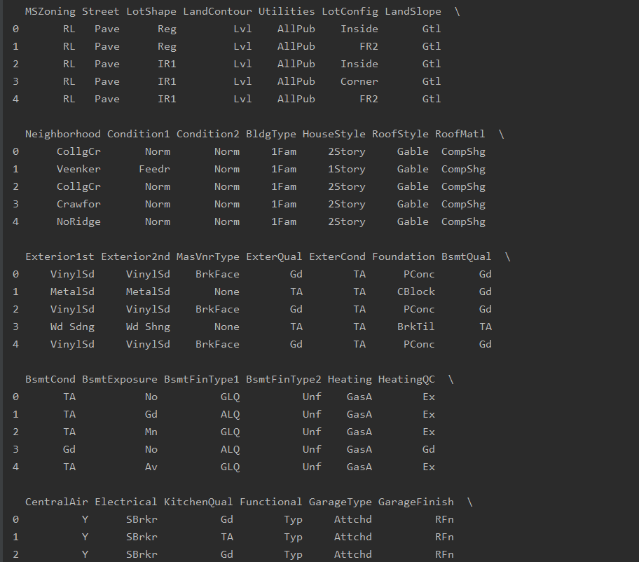
六:实例化独热编码对象
6-1 实例化独热编码对象 获取列名
# 实例化独热编码对象
OneHot = OneHotEncoder()
# numpy ndarray
result = OneHot.fit_transform(ob_df_data).toarray()
# 获取列名
OneHotNames = OneHot.get_feature_names().tolist()
print(OneHotNames, len(OneHotNames))
输出结果如下,共计234列的列名

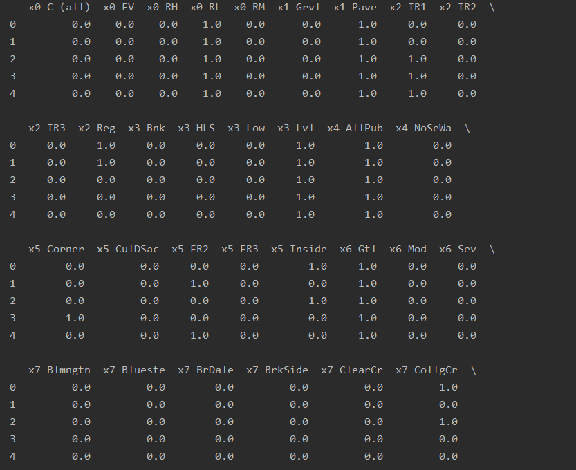
6-2 独热编码过后的DataFrame 【字符列转数字列】
# 独热编码过后的dataframe
OneHot_df = pd.DataFrame(result, columns=OneHotNames)
print(OneHot_df.head())
查看全部的独热编码后的dataframe
6-3 删除原来的38列字符数据、行合并
# 删除原来的38列字符数据  75-38=37
data_df.drop(columns=ob_feature, inplace=True)
# 行合并 37+234[独热编码出来的新列]=271列+label列=272
data_df = pd.concat([OneHot_df, data_df], axis=1)
print(data_df.head(), data_df.shape)  # (1460, 272)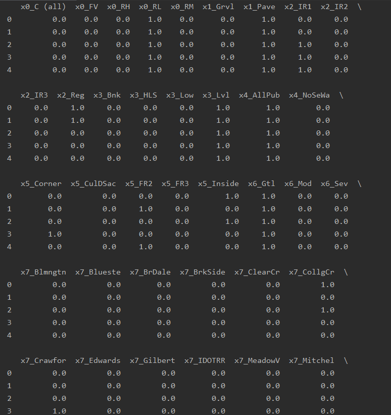
得出结果(1460, 272) ,即以上操作的规模为1460行、272列,
feature特征数据太多了,计算量太大,需要解决这个问题
七:方差过滤
方差过滤(方差小于0.1进行过滤) + 数据提纯
# feature太多 计算量过大
# 方差过滤
var_index = VarianceThreshold(threshold=0.1)
data = var_index.fit_transform(data_df)
# 获取留下了的索引
index = var_index.get_support(True).tolist()
# print(index)
data_df = data_df.iloc[:, index]
print(data_df.head(), data_df.shape) # (1460, 84)数据量降低处理操作:由272降至84
(1460, 84)八:特征数据提取
# 相关系数分析--皮尔逊相关系数(根据权重)
features = data_df.columns.tolist()
# print(features)

f_names = []  # pearsonr>0.5的列名
# 每一列都要计算与最后一列的pearsonr>0.5
for i in range(0, len(features)):
    if abs(pearsonr(data_df[features[i]], data_df[features[-1]])[0]) > 0.5:
        f_names.append(features[i])
print(f_names, len(f_names)) # 14数据量降低处理操作:由84降至14
['x17_TA', 'x29_TA', 'x32_Unf', 'OverallQual', 'YearBuilt', 'YearRemodAdd', 'TotalBsmtSF', '1stFlrSF', 'GrLivArea', 'FullBath', 'TotRmsAbvGrd', 'GarageCars', 'GarageArea', 'SalePrice'] 14九:查看特征之间的相关系数
f_names = []  # pearsonr>0.5的列名
# 存储皮尔逊相关系数的值
pear_num = []
# 每一列都要计算与最后一列的pearsonr>0.5
for i in range(0, len(features) - 1):
    if abs(pearsonr(data_df[features[i]], data_df[features[-1]])[0]) > 0.5:
        f_names.append(features[i])
        pear_num.append(pearsonr(data_df[features[i]], data_df[features[-1]])[0])
# print(f_names, len(f_names))  # 13

# 查看特征之间的相关系数
import matplotlib.pyplot as plt
import seaborn as sns

# 根据相关系数的大小--数据封装,封装成DataFrame
pear_dict = {
    'features': f_names,
    'pearData': pear_num
}
hotPear = pd.DataFrame(pear_dict)
print(hotPear)
features pearData
0 x17_TA -0.589044
1 x29_TA -0.519298
2 x32_Unf -0.513906
3 OverallQual 0.790982
4 YearBuilt 0.522897
5 YearRemodAdd 0.507101
6 TotalBsmtSF 0.613581
7 1stFlrSF 0.605852
8 GrLivArea 0.708624
9 FullBath 0.560664
10 TotRmsAbvGrd 0.533723
11 GarageCars 0.640409
12 GarageArea 0.623431十:皮尔逊系数重排
# 皮尔逊相关系数按照从大到小
hotPear.sort_values(by=['pearData'], ascending=False, inplace=True)
# 重置index
hotPear.reset_index(drop=True, inplace=True)
print(hotPear)
features pearData
0 OverallQual 0.790982
1 GrLivArea 0.708624
2 GarageCars 0.640409
3 GarageArea 0.623431
4 TotalBsmtSF 0.613581
5 1stFlrSF 0.605852
6 FullBath 0.560664
7 TotRmsAbvGrd 0.533723
8 YearBuilt 0.522897
9 YearRemodAdd 0.507101
10 x32_Unf -0.513906
11 x29_TA -0.519298
12 x17_TA -0.589044十一:热力图绘制
首先,热力图相关安装命令如下,pip install seaborn,没有安装过的可以先安装一下
# 开始绘图
plt.figure(figsize=(12, 12))
sns.set(font_scale=0.8)
cor = np.corrcoef(data_df[f_names].values.T)
# 数据填充
sns.heatmap(cor, cbar=False, annot=True, square=True, fmt='0.2f', yticklabels=f_names,
            xticklabels=f_names)
plt.show()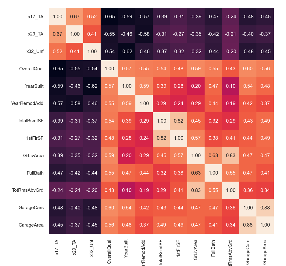
分析出相似度极高的列名组合,
需要舍弃相似度高的列组合其中的某一列
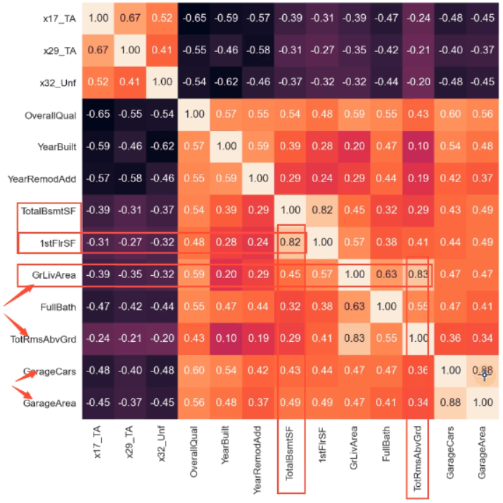
如上图,分析得出:
需要舍弃包括有如下三组(相似度超过80)
GarageArea GarageCars  88
TotRmsAbvGrd GrLivArea 83
1stFIrSF TotalBsmtSF   82
# 舍弃相似度高的三列
f_names.append("SalePrice")
data_df = data_df[f_names]
data_df.drop(['GarageArea', 'TotRmsAbvGrd', '1stFlrSF'], inplace=True, axis=1)
print(data_df.head(), data_df.shape)数据量降低处理操作:由14降至11,除去标签列,特征列为10列
(1460, 11)十二:数据集划分
from sklearn.model_selection import train_test_split
from sklearn.preprocessing import StandardScaler

# 分出feature->array  label->array
feature_data = data_df.iloc[:, :-1].values
# print(type(feature_data))
label_data = np.ravel(data_df.iloc[:, -1].values)
# print(label_data,type(label_data))
X_train, X_test, y_train, y_test = train_test_split(feature_data, label_data, test_size=0.3, random_state=666)
std = StandardScaler()
X_train_std = std.fit_transform(X_train)
X_test_std = std.fit_transform(X_test)
print(X_train_std)
[[ 0.78554988 1. 1.05431032 ... -0.97998523 -1.0304426
-0.98880127]
[ 0.78554988 1. 1.05431032 ... -1.1228905 -1.0304426
-0.98880127]
[ 0.78554988 -1. 1.05431032 ... -0.27879671 -1.0304426
-2.28771502]
...
[ 0.78554988 1. -0.94848735 ... -0.20829678 -1.0304426
0.31011248]
[ 0.78554988 1. 1.05431032 ... -0.68845848 -1.0304426
-2.28771502]
[-1.27299365 -1. -0.94848735 ... -0.1663779 0.80424788
0.31011248]]十三:网格模型 超参调优
from sklearn.model_selection import train_test_split, GridSearchCV
from sklearn.preprocessing import StandardScaler
from sklearn.neighbors import KNeighborsRegressor
model = KNeighborsRegressor()
param_list = [
{
'n_neighbors': list(range(1, 38)),
'weights': ['uniform']
},
{
'n_neighbors': list(range(1, 38)),
'weights': ['distance'],
'p': [i for i in range(1, 21)]
}
]
grid = GridSearchCV(model, param_grid=param_list, cv=10)
grid.fit(X_train_std, y_train)
print(grid.best_score_)
print(grid.best_params_)
print(grid.best_estimator_)
best_model = grid.best_estimator_输出如下结果,程序跑的时间有点长,需要耐心等待
0.8368525468413448
{'n_neighbors': 13, 'p': 1, 'weights': 'distance'}
KNeighborsRegressor(n_neighbors=13, p=1, weights='distance')
十四:训练模型 预测实际比对
best_model = KNeighborsRegressor(n_neighbors=13, p=1, weights='distance')
# 训练模型
best_model.fit(X_train_std, y_train)
# 模型保存
import joblib
joblib.dump(best_model, "PriceRegModel.model")
# 预测
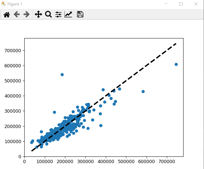
y_predict = best_model.predict(X_test_std)
# 预测与实际 图示点状图
plt.scatter(y_test, y_predict, label="test")
plt.plot([y_test.min(), y_test.max()],
[y_test.min(), y_test.max()],
'k--',
lw=3,
label="predict"
)
plt.show()模型保存
预测实际比对
十五:完整源码分享
from sklearn.impute import SimpleImputer  # 众数
from sklearn.preprocessing import OneHotEncoder  # 独热编码
from sklearn.feature_selection import VarianceThreshold  # 方差过滤
from scipy.stats import pearsonr  # 皮尔逊相关系数
import pandas as pd
import numpy as np

# 设置显示所有行、列
pd.set_option("display.max_rows", None)
pd.set_option("display.max_columns", None)
data_df = pd.read_csv("train.csv", sep=',')
# print(data_df.head(), data_df.shape)  # 1460*80

# 空值处理
# print(data_df.isnull().sum())
# 超过1/3列的剔除
data_df.drop(columns=['Alley', 'FireplaceQu', 'PoolQC', 'Fence', 'MiscFeature'],
             axis=1, inplace=True)
# print(data_df.shape)

# 2 空值填充
# 2-1 [数字列]填充
data_df['LotFrontage'].fillna(data_df['LotFrontage'].mean(), inplace=True)
data_df['GarageYrBlt'].fillna(data_df['GarageYrBlt'].median(), inplace=True)
data_df['MasVnrArea'].fillna(data_df['MasVnrArea'].median(), inplace=True)
# print(data_df.isnull().sum())

# 2-2 剩余的[字符列]在miss_col_list中
# 获取缺失列的名字
miss_col_list = data_df.isnull().any()[data_df.isnull().any().values == True].index.tolist()
# print(data_df.isnull().any())
# print(miss_col_list)

# 获取缺失列对应的列值--list
miss_list = []

for i in miss_col_list:
    miss_list.append(data_df[i].values.reshape(-1, 1))  # 任意行 列数为1
# print(miss_list)

# 对每一列进行众数填充
for i in range(0, len(miss_list)):
    im_most = SimpleImputer(strategy='most_frequent')
    most = im_most.fit_transform(miss_list[i])
    data_df.loc[:, miss_col_list[i]] = most

# print(data_df.isnull().sum())

# 目标找到所有的字符列
ob_feature = data_df.select_dtypes(include=['object']).columns.tolist()
# print(ob_feature, len(ob_feature))
ob_df_data = data_df.loc[:, ob_feature]
# print(ob_df_data.head())

# 实例化独热编码对象
OneHot = OneHotEncoder()
# numpy ndarray
result = OneHot.fit_transform(ob_df_data).toarray()
# 获取列名
OneHotNames = OneHot.get_feature_names().tolist()
# print(OneHotNames, len(OneHotNames))

# 独热编码过后的dataframe
OneHot_df = pd.DataFrame(result, columns=OneHotNames)
# print(OneHot_df.head())

# 删除原来的38列字符数据  75-38=37
data_df.drop(columns=ob_feature, inplace=True)
# 行合并 37+234[独热编码出来的新列]=271列+label列=272
data_df = pd.concat([OneHot_df, data_df], axis=1)
# print(data_df.head(), data_df.shape)  # (1460, 272)

# feature太多 计算量过大
# 方差过滤
var_index = VarianceThreshold(threshold=0.1)
data = var_index.fit_transform(data_df)
# 获取留下了的索引
index = var_index.get_support(True).tolist()
# print(index)
data_df = data_df.iloc[:, index]
# print(data_df.head(), data_df.shape)  # (1460, 84)

# 相关系数分析--皮尔逊相关系数(根据权重)
features = data_df.columns.tolist()
# print(features)

f_names = []  # pearsonr>0.5的列名
# 存储皮尔逊相关系数的值
pear_num = []
# 每一列都要计算与最后一列的pearsonr>0.5
for i in range(0, len(features) - 1):
    if abs(pearsonr(data_df[features[i]], data_df[features[-1]])[0]) > 0.5:
        f_names.append(features[i])
        pear_num.append(pearsonr(data_df[features[i]], data_df[features[-1]])[0])
# print(f_names, len(f_names))  # 13

# 查看特征之间的相关系数
import matplotlib.pyplot as plt
import seaborn as sns

# 根据相关系数的大小--数据封装,封装成DataFrame
pear_dict = {
    'features': f_names,
    'pearData': pear_num
}
hotPear = pd.DataFrame(pear_dict)
# print(hotPear)

# 皮尔逊相关系数按照从大到小
hotPear.sort_values(by=['pearData'], ascending=False, inplace=True)
# 重置index
hotPear.reset_index(drop=True, inplace=True)
# print(hotPear)

# # 开始绘图
# plt.figure(figsize=(12, 12))
# sns.set(font_scale=0.8)
# cor = np.corrcoef(data_df[f_names].values.T)
# # 数据填充
# sns.heatmap(cor, cbar=False, annot=True, square=True, fmt='0.2f', yticklabels=f_names,
#             xticklabels=f_names)
# # plt.show()

#  舍弃相似度高的三列
f_names.append("SalePrice")
data_df = data_df[f_names]
data_df.drop(['GarageArea', 'TotRmsAbvGrd', '1stFlrSF'], inplace=True, axis=1)
# print(data_df.head(), data_df.shape)

from sklearn.model_selection import train_test_split, GridSearchCV
from sklearn.preprocessing import StandardScaler
from sklearn.neighbors import KNeighborsRegressor

# 分出feature->array  label->array
feature_data = data_df.iloc[:, :-1].values
# print(type(feature_data))
label_data = np.ravel(data_df.iloc[:, -1].values)
# print(label_data,type(label_data))
X_train, X_test, y_train, y_test = train_test_split(feature_data, label_data, test_size=0.3, random_state=666)
std = StandardScaler()
X_train_std = std.fit_transform(X_train)
X_test_std = std.fit_transform(X_test)
# print(X_train_std)

# model = KNeighborsRegressor()
# param_list = [
#     {
#         'n_neighbors': list(range(1, 38)),
#         'weights': ['uniform']
#     },
#     {
#         'n_neighbors': list(range(1, 38)),
#         'weights': ['distance'],
#         'p': [i for i in range(1, 21)]
#     }
# ]
# grid = GridSearchCV(model, param_grid=param_list, cv=10)
# grid.fit(X_train_std, y_train)
# print(grid.best_score_)
# print(grid.best_params_)
# print(grid.best_estimator_)
# best_model = grid.best_estimator_

best_model = KNeighborsRegressor(n_neighbors=13, p=1, weights='distance')
# 训练模型
best_model.fit(X_train_std, y_train)
# 模型保存
import joblib

joblib.dump(best_model, "PriceRegModel.model")

# 预测
y_predict = best_model.predict(X_test_std)
# 预测与实际 图示点状图
plt.scatter(y_test, y_predict, label="test")
plt.plot([y_test.min(), y_test.max()],
         [y_test.min(), y_test.max()],
         'k--',
         lw=3,
         label="predict"
         )
plt.show()
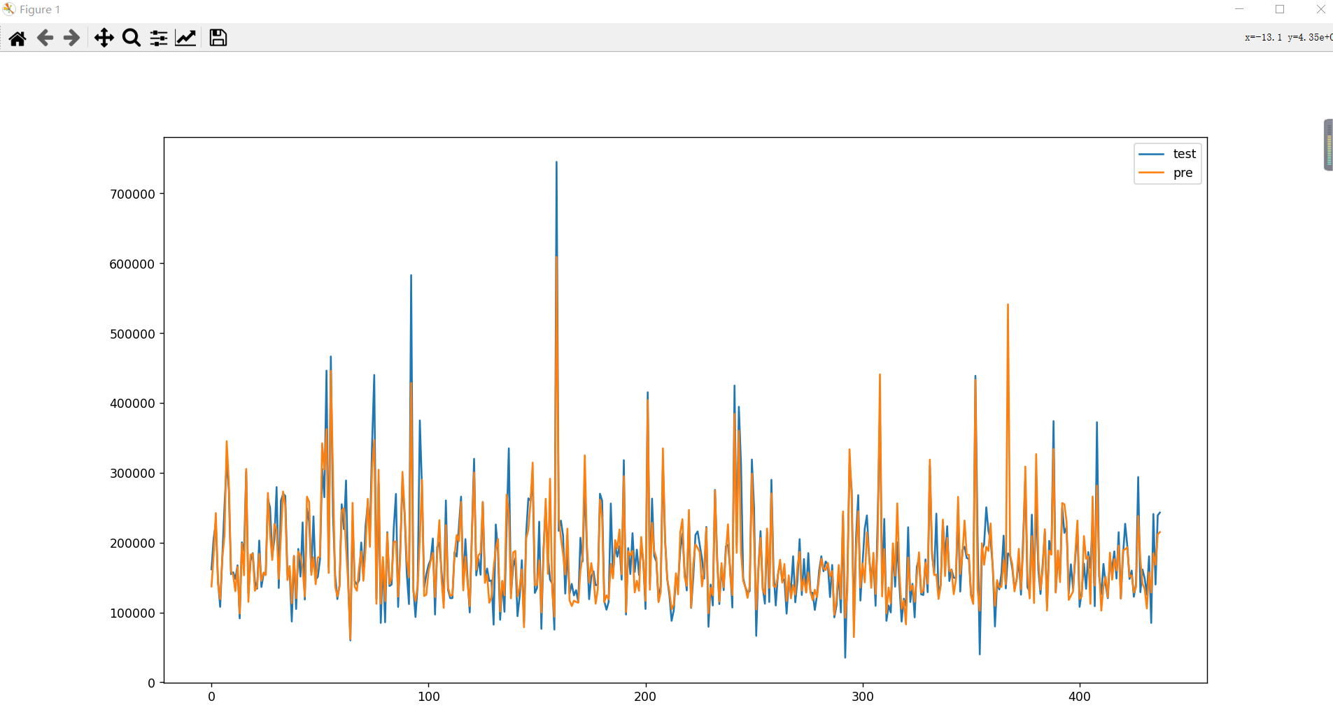
预测实际比对,也可以使用线型图方式查看
test_pre = pd.DataFrame({"test": y_test.tolist(),
                         "pre": y_predict.flatten()
                         })
test_pre.plot(figsize=(18, 10))
plt.show()